Here there are two parts:
- Diffusion model implementation
- Vision Transformer based Diffusion Model Implementation
For the diffusion model implementation (DDPM), see the other blog post . In this blogpost, we look at the implementation of latent diffusion model with transformer backbone, in particular from the DiT Paper with its Github repository .
In the notation here, the shapes are by convention:
- $B$: batch size.
- $H$: height of image.
- $W$: weight of image.
- $C_{in}$: input channel, $C$ for channel number in general.
- $D$: usually for the embedding dimension (output)
Diffusion Part
The general paradigm in this line of work is known as latent diffusion models, which maps the original data samples (images in this case) into a latent space of lower dimension $Z$, then conduct diffusion in the latent space.
DiT Implementation
For the input image processing, timm.models.vision_transformer is used, with PatchEmbed, Attention, and Mlp modules used. In particular, PatchEmbed is used to handle the input image: this is the technique used by vision transformer to turn a 2D image into a sequence of patch tokens.
Conditional Contextual Embeddings
In order to perform conditional generation, DiT incorporates inputs in addition to the input image. The DiT model also use:
- time step $t$: this corresponds to the time index of the diffusion step.
- label $y$: this corresponds to the label of the image. Optionally, input can also contain embeddings for natural languages that serve as context.
DiT.models.TimeStepEmbedder (L27-64) handles the embedding of input time tensor of size $(B,)$, one for each batch element and outputs a $(B,D)$. It uses sinusoidal timestep embedding followed by a MLP, which can be used as a generic way to do time step embedding.
DiT.models.LabelEmbedder (L67-95) handles the embedding of labels. It handles both classifier and classifier-free guidance (by randomly dropping this embedding, using the class_dropout_prob parameter from the DiT class). The embedding is simply handled with an nn.Embedding(num_classes + use_cfg_embedding, hidden_size) layer.
From the DiT implementation, they only use labels for classifier free guidance, and time index embedding is always used.
DiT Block
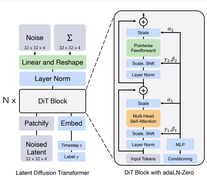
DiT.models.DiTBlock (L101-123) contains the code for this block.
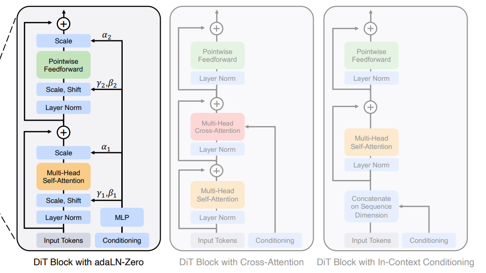
The details about the DiT block is in Figure 3 of the DiT Paper:

We can see that there are two data paths:
- The input tokens (patchified noise latent) is fed into the main transformer blocks.
- The conditioning (embeddings from time and label) is fed into a MLP, then to the input and output of the transformer block.
The forward pass is quite straightforward: what’s a little less intuitive is that a MLP that takes conditional embeddings is used to generate transformation parameters (translation, shift, scale) applied to the image before feeding into the attention and MLP components.
def modulate(x, shift, scale):
    return x * (1 + scale.unsqueeze(1)) + shift.unsqueeze(1)

def forward(self, x, c):
    # handling of contextual embeddings: generate transformation variables for attention and mlp
    shift_msa, scale_msa, gate_msa, shift_mlp, scale_mlp, gate_mlp = self.adaLN_modulation(c).chunk(6, dim=1)
    # handling of x: transform x then feed into mlp and attention modules.
    x = x + gate_msa.unsqueeze(1) * self.attn(modulate(self.norm1(x), shift_msa, scale_msa))
    x = x + gate_mlp.unsqueeze(1) * self.mlp(modulate(self.norm2(x), shift_mlp, scale_mlp))
    return x
Then the Final Layer of DiT (L125-142) is simply the version of DiT block without the attention part
DiT Module
The DiT module itself is a stacking of multiple DiT blocks followed by the final layer.

def forward(self, x, t, y):
    """
    Forward pass of DiT.
    x: (N, C, H, W) tensor of spatial inputs (images or latent representations of images)
    t: (N,) tensor of diffusion timesteps
    y: (N,) tensor of class labels
    """
    x = self.x_embedder(x) + self.pos_embed  # (N, T, D), where T = H * W / patch_size ** 2
    t = self.t_embedder(t)                   # (N, D)
    y = self.y_embedder(y, self.training)    # (N, D)
    c = t + y                                # (N, D)
    for block in self.blocks:
        x = block(x, c)                      # (N, T, D)
    x = self.final_layer(x, c)                # (N, T, patch_size ** 2 * out_channels)
    x = self.unpatchify(x)                   # (N, out_channels, H, W)
    return x
one additional detail, as customary from vision transformers, is that input image after patchfying also has sine cosine positional embeddings (called frequency embedding).
For the classifier-free guidance based forward pass, a different forward pass is used:
def forward_with_cfg(self, x, t, y, cfg_scale):
    """
    Forward pass of DiT, but also batches the unconditional forward pass for classifier-free guidance.
    """
    # https://github.com/openai/glide-text2im/blob/main/notebooks/text2im.ipynb
    half = x[: len(x) // 2]
    combined = torch.cat([half, half], dim=0)
    model_out = self.forward(combined, t, y)
    # For exact reproducibility reasons, we apply classifier-free guidance on only
    # three channels by default. The standard approach to cfg applies it to all channels.
    # This can be done by uncommenting the following line and commenting-out the line following that.
    # eps, rest = model_out[:, :self.in_channels], model_out[:, self.in_channels:]
    eps, rest = model_out[:, :3], model_out[:, 3:]
    cond_eps, uncond_eps = torch.split(eps, len(eps) // 2, dim=0)
    half_eps = uncond_eps + cfg_scale * (cond_eps - uncond_eps)
    eps = torch.cat([half_eps, half_eps], dim=0)
    return torch.cat([eps, rest], dim=1)
with the standard random dropping of conditions from inputs (in this case they use a fancier way to do it). In particular, as laid out in section 3 of the paper, the output from the noise network can be framed as:
$$\begin{align} \hat{\epsilon}_{\theta} (x_t, c) = \epsilon_{\theta}(x_t, \emptyset) + s \cdot \nabla_{x} \log p(x\mid c) \propto \epsilon_{\theta} (x_t, \emptyset) + s \cdot (\epsilon_{\theta}(x_t, c) - \epsilon_{\theta}(x_{t}, \emptyset)) \end{align}$$
where the conditional information $c$ is randomly dropped (denoted $\emptyset$ in this case). Key steps are in the p_sample function (L376-417) for DDPM based sampling. To control this conditional information masking, the DiT model’s constructor has the parameter of class_drop_pro which is then used by the LabelEmbedder class.
Diffusion Implementation
The diffusion code is in DiT.diffusion.gaussian_diffusion.py, where the entry point to this module is in DiT.diffusion.__init__.py, where the main diffusion model is set to be the SpaceDiffusion model in DiT.diffusion.respace.py, which inherts from DiT.diffusion.gaussian_diffusion.GaussianDiffusion, only changing the forward diffusion schedule (beta values and number of time steps).
Latent Encoding
Since the DiT belongs to the class of models known as latent diffusion models, first the input must be encoded into a latent space. This is achieved in L203 in DiT.train.py:
# declaration of VAE
from diffusers.models import AutoencoderKL
vae = AutoencoderKL.from_pretrained(f"stabilityai/sd-vae-ft-{args.vae}").to(device)
# L203
# Map input images to latent space + normalize latents:
x = vae.encode(x).latent_dist.sample().mul_(0.18215)
Latent Decoding
From DiT.sample_ddp.py and DiT.sample.py, vae.decode is used to convert the latent representation to the image space:
# sample_ddp.py L 131-132
samples = vae.decode(samples / 0.18215).sample
samples = torch.clamp(127.5 * samples + 128.0, 0, 255).permute(0, 2, 3, 1).to("cpu", dtype=torch.uint8).numpy()

# sample.py L64-65
samples, _ = samples.chunk(2, dim=0)  # Remove null class samples
samples = vae.decode(samples / 0.18215).sample
GaussianDiffusion
Training: training_losses
The implementation of the GaussianDiffusion class in DiT.diffusion.gaussian_diffusion.py differ from the DDPM repository, as covered in another post
. This implmentation was done approximately one year after the original DDPM paper, so the code layout looks cleaner and more readable.
member functions q_mean_variance, q_sample, q_posterior_mean_variance are about the same as in original DDPM. The main training function training_losses (L715-787) contains 3 different choices of loss functions:
- KL type loss and rescaled KL type loss.
- MSE and rescaled MSE loss.
where the KL type losses are implemented in _vb_terms_bpd function (L682-713). This function computes the ELBO using x_t, x_0, and t, by the following equation on section 3.1 in the DiT paper:
$$\begin{align} \mathcal{L}(\theta) = -p(x_0 \mid x_1) + \sum_{t} \mathcal{D}_{KL}(q^{\ast}(x_{t-1}\mid x_t, x_0) \mid \mid p_{\theta}(x_{t-1}\mid x_t)) \end{align}$$
Then for the MSE based loss, it refers to the loss for the paramterized noise network $\epsilon_\theta$, with the “simple loss” termed in section 3.1 of the DiT paper:
$$\begin{align} \mathcal{L}_{\text{simple}}(\theta) = \mid \mid \epsilon_{\theta}(x_{t}) - \epsilon_{t} \mid \mid_{2}^2 \end{align}$$
and the loss in the end is a combination of these two loss terms.
Inference: DDIM Sampling + DDPM Sampling
The crucial function for sampling in this case is the p_mean_variance function (L254-333), which computes $p(x_{t-1}\mid x_t)$, predicted $x_t, x_0$, which can be used to compute the samples straightforwardly (as in DDPM, function p_sample) or using a shorter sampling trajectory (DDIM, as in ddim_sample). The implementation in general is similar to the one in the DDPM codebase, with complications from design choices that are a little difficult to read.
TBD: Design Choices and Tricks
As with other vision models, this model contains many design tricks and choices that are not directly talked about in the paper. (to be udpated).