A Unified Uncertainty Representation for Graph Neural Networks
DSS-GNN stores each node’s embedding as a short polynomial chaos expansion in one shared Gaussian variable and filters it along two spectral axes, graph frequency and chaos order. Readouts of this one representation, computed in a single deterministic pass, give calibrated predictions, OOD scores and robustness to distribution shift.
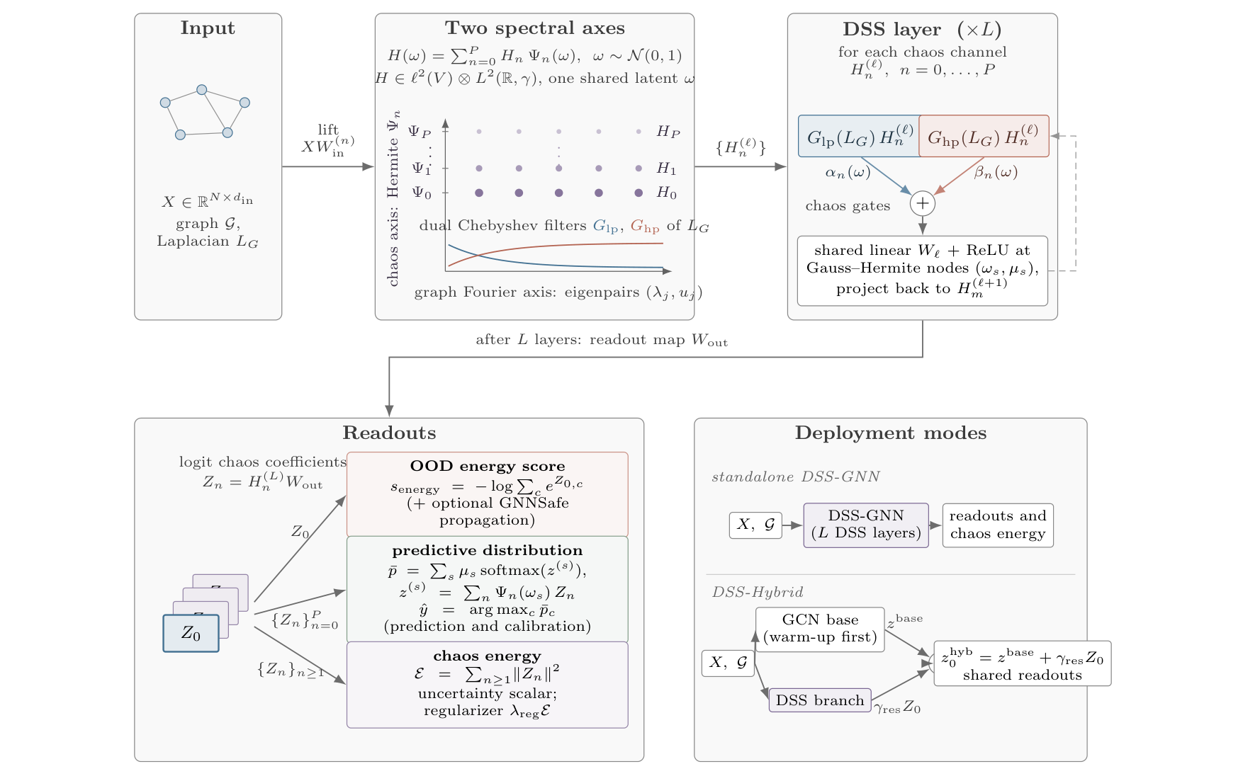
This post introduces our NeurIPS 2026 paper, “A Unified Uncertainty Representation for Graph Neural Networks via Doubly-Spectral Stochastic Expansion,” written with Thomas Markovich of Block, Florence Regol of Mila and Yizhou Sun of UCLA. A graph neural network that is used for real decisions should do three things besides predicting: give probabilities that match how often it is right, which is calibration; recognize inputs unlike its training data, which is out-of-distribution or OOD detection; and keep its accuracy when the data changes, which is robustness to distribution shift. Existing methods usually address one of these with a dedicated model. DSS-GNN instead stores, for every node, a short polynomial expansion in a single Gaussian random variable rather than one fixed vector, and filters this expansion along two spectral axes, graph frequency and chaos order, so that different readouts of one representation, all computed in a single deterministic forward pass, serve the three tasks. On its own, DSS-GNN has the lowest Brier score among the compared uncertainty-aware methods on all 14 node classification benchmarks; added as a residual branch to a standard GCN, which we call DSS-Hybrid, it has the best OOD AUROC among the compared methods on 6 of 9 node-level settings and, trained with plain empirical risk minimization, the highest accuracy on all 7 GOOD concept-shift benchmarks.
Why a graph neural network should say how sure it is
Many datasets are networks, in which molecules are atoms connected by bonds, a payment platform is accounts connected by transactions, and a road system is intersections connected by roads. Each node has features, such as the words on a web page or an account’s history, while edges say which nodes are related, and a graph neural network, or GNN, predicts something about each node, such as its class, by combining the node’s own features with those of its neighbors. GNNs now appear in drug discovery, fraud detection and traffic forecasting, settings in which a wrong answer given with high confidence is often worse than an answer that says “I am not sure,” and a deployed model should therefore satisfy three requirements.
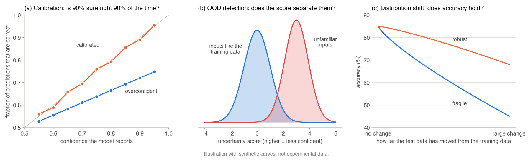
We measure them with standard numbers. The Brier score, the average squared difference between the predicted class probabilities and the true answer written as a 0/1 vector, measures calibration and accuracy together, so that a model is penalized both for being wrong and for being more or less confident than it should be, and lower is better. AUROC measures OOD detection as the probability that a randomly chosen OOD node gets a higher “unfamiliar” score than a randomly chosen in-distribution node, so that 50 is chance and 100 is perfect. And shifted accuracy is plain accuracy measured on test data drawn from a different distribution than the training data.
On graphs the three requirements are linked, because how certain a prediction should be depends on the node’s neighborhood as well as on its own features, and all three are versions of one question, when and how confidently the model can predict. Yet most existing methods target only one of them. Sampling methods such as MC-dropout and Deep Ensembles run the model many times; evidential models such as GPN give OOD evidence but not shift-robust classification; energy-based detectors give scores that separate familiar from unfamiliar inputs but not calibrated probabilities; and robust-training methods do not model uncertainty explicitly. Our goal was a single representation of uncertainty inside the GNN, from which each task reads what it needs, and to build it we combine two mathematical tools that are each well established, spectral graph theory and polynomial chaos, which the next four sections introduce.
Signals on a graph and their frequencies
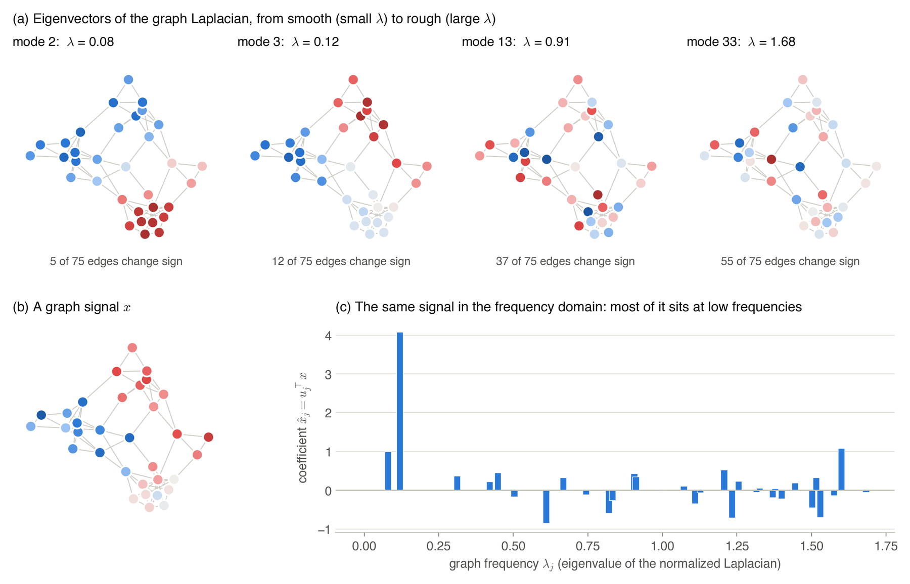
Take a graph with nodes. A graph signal assigns one number to each node, so it is a vector , and a node feature, such as how often the word learning appears on a web page, is a graph signal, as is each coordinate of a GNN’s hidden representation. The set of all graph signals is a vector space, written , with the usual inner product , which means that we can add signals, scale them, measure their length and, most importantly, write every signal in a basis.
The basis that respects the graph comes from the graph Laplacian, which in its simplest form is , where is the adjacency matrix and the diagonal matrix of node degrees. For any signal,
which is small when connected nodes have similar values and large when they do not. Spectral GNNs usually work with a normalized Laplacian, such as , which has the same interpretation and eigenvalues between 0 and 2.
Because is symmetric, its eigenvectors form an orthonormal basis of . Each eigenvector is itself a graph signal, and its eigenvalue measures how much that signal changes across edges, so that the eigenvectors play the role that sines and cosines play for sound: a small means a smooth, slowly varying pattern, a low frequency, and a large one a pattern that changes sign across many edges, a high frequency. Any signal can be written as
and the coefficients are its graph Fourier transform. Because the basis is orthonormal, the squared length of the signal is the sum of the squared coefficients, .
Filtering a signal on a graph
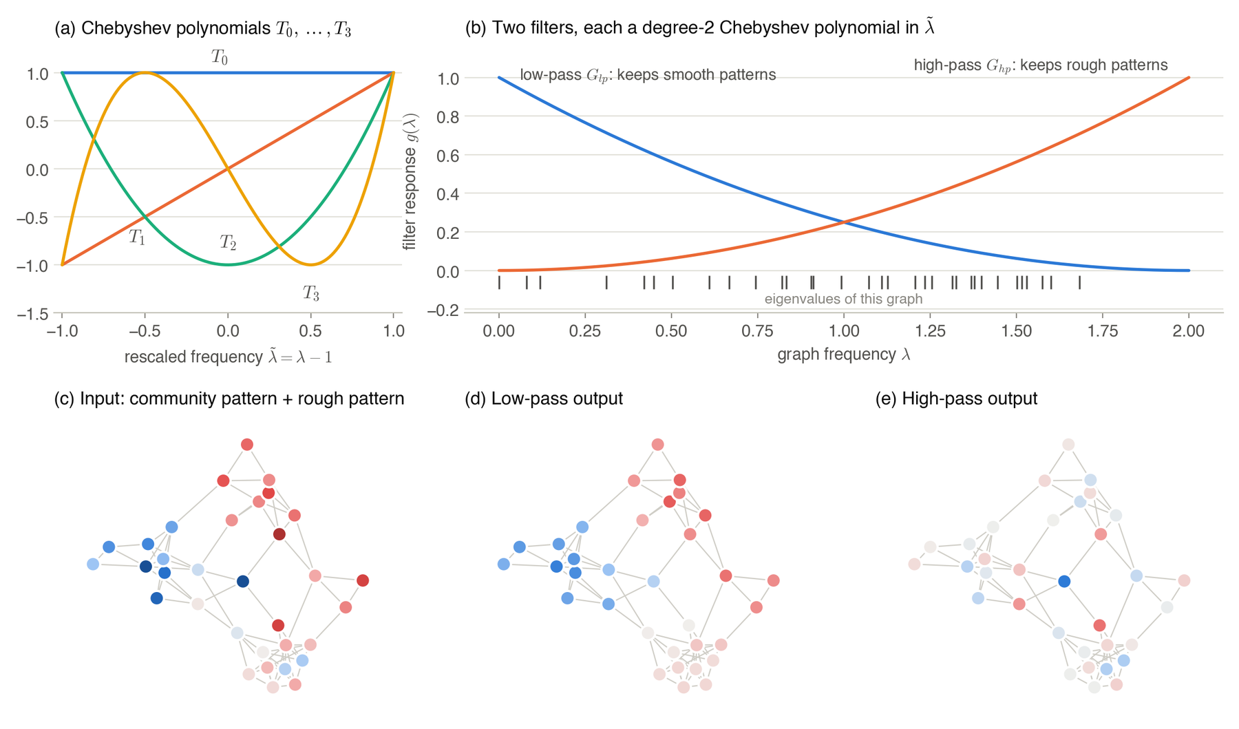
On a regular grid, convolution is the same as multiplication in the Fourier domain, and because a graph has no notion of shifting a pattern from one place to another, spectral GNNs turn this property into the definition of convolution on a graph. A spectral filter changes how much of each frequency a signal contains, multiplying the coefficient by a number and transforming back, so that in matrix form the output is . Computing all the eigenvectors of a large graph is expensive, so spectral GNNs choose to be a polynomial, which needs only repeated multiplication by , and a polynomial of degree combines information from neighbors at most edges away. ChebNet, a standard spectral GNN, writes the polynomial in the Chebyshev basis,
where , and , and the coefficients are learned. The rescaling moves the eigenvalues into , where Chebyshev polynomials are well behaved, staying bounded by 1 and giving close to the best polynomial approximation of a given degree, and GCN is the special case of a first-order Chebyshev filter with a single shared coefficient.
Two kinds of filter matter here. A low-pass filter keeps smooth patterns and removes rough ones, which suits graphs where neighbors tend to share labels, a property called homophily that holds for citation networks, while a high-pass filter keeps the differences between neighbors and is useful when neighbors tend to differ, which is heterophily. DSS-GNN applies both a low-pass and a high-pass Chebyshev filter in every layer, so it can learn which frequencies matter on each graph.
Random quantities as functions of a Gaussian
So far everything has been deterministic. To represent uncertainty we want each node’s hidden representation to be a random quantity rather than a fixed vector, and the question is how to store a random quantity with a finite list of numbers. The approach we use, called polynomial chaos, starts from one standard Gaussian variable and writes the random quantity as a function of it, : , for example, is a Gaussian with mean and standard deviation , while is a skewed, always positive random quantity.
There are several ways to give a neural network a random representation, and each has a cost. Sampling methods such as MC-dropout and Deep Ensembles represent uncertainty by many forward passes or many models, which multiplies the cost and adds sampling noise to every estimate; parametric methods give each embedding a mean and a variance, which is cheap but describes only Gaussians, and a nonlinearity such as ReLU destroys the Gaussian form after a single layer; and evidential methods put a distribution on the class probabilities at the output but leave the hidden representation deterministic. Polynomial chaos takes a different route, borrowed from uncertainty quantification in engineering, where since the stochastic finite element methods of Ghanem and Spanos in 1991 it has been the standard way to push random inputs through physical simulations. It represents a random quantity by the coefficients of an orthogonal expansion, much as a Fourier series represents a function, so that the mean and the variance can be read off the coefficients in closed form, non-Gaussian shapes need only a few more coefficients, and every computation, nonlinear ones included, can be carried out deterministically by quadrature rather than by sampling.
The functions with finite variance, , form a vector space written , where is the Gaussian distribution. It has an inner product, , exactly as graph signals do, the difference being that this space is infinite-dimensional, and it too has a natural orthogonal basis, the Hermite polynomials,
and so on, generated by the recurrence . After normalizing, , they satisfy
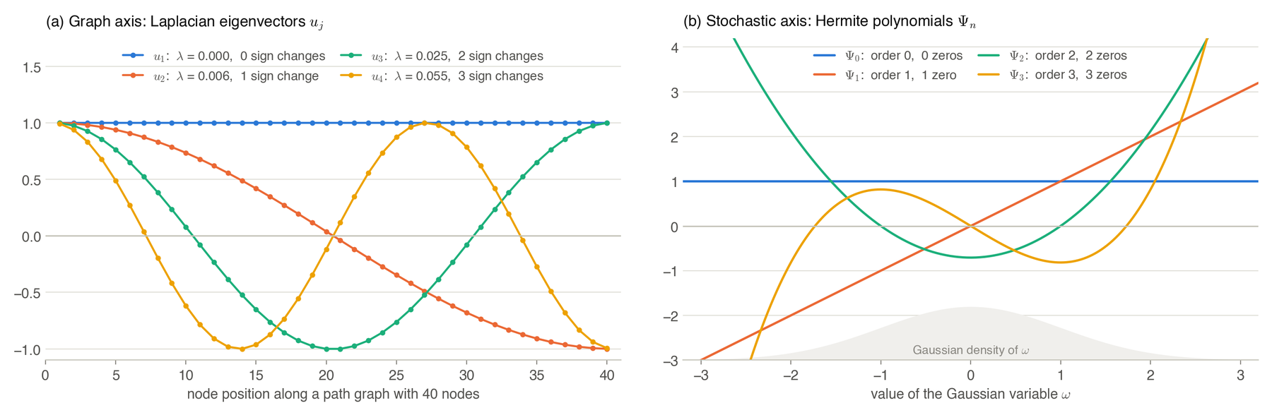
The parallel with the graph is closer than it might look. The Laplacian eigenvectors are sorted by eigenvalue, and the -th one on a path graph changes sign times, while the Hermite polynomials are sorted by order , and has zeros. Both families are eigenvectors of a symmetric operator, on the graph and for the Ornstein–Uhlenbeck operator on , so the chaos order plays the role of a frequency for randomness. The Gaussian is not the only possible base variable, since generalized polynomial chaos pairs other distributions with their own orthogonal polynomials, Legendre polynomials for a uniform variable for instance, but the Gaussian and its Hermite polynomials are the classical choice, the one Wiener introduced, and the one whose quadrature rule we will use.
The polynomial chaos expansion
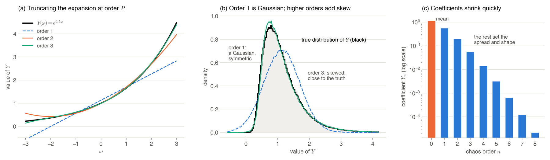
Because the Hermite polynomials form a complete orthonormal basis, a classical result of Wiener and of Cameron and Martin, every finite-variance function of can be written as
This is the polynomial chaos expansion, where “chaos” is Wiener’s historical name and has nothing to do with chaotic dynamics. Two facts make it useful for uncertainty: the mean is the first coefficient, , because and every other has mean zero, and the variance is the sum of the squared remaining coefficients, , a quantity we call the chaos energy.
In practice we keep only the terms up to order . With , , which is exactly a Gaussian, while with the expansion can also describe skewed or otherwise non-Gaussian quantities. For sufficiently regular functions the coefficients shrink quickly with , exponentially fast under the smoothness condition of the paper’s Theorem 2, so a small is often enough.
Two axes at once: the doubly-spectral expansion
Now we combine the two ideas. A random graph signal assigns a random quantity to each node, and in DSS-GNN all the randomness comes from one shared Gaussian variable , so that every node’s value is a function of the same . This is a deliberate simplification: a single variable keeps every average over the randomness one-dimensional, so that a handful of quadrature points computes it exactly, and it makes the variations of neighboring nodes move together, a limitation we return to at the end. Such signals are the elements of the product space , and the products of a graph eigenvector and a Hermite polynomial form a complete orthonormal basis of it, so that every such signal has a doubly-spectral stochastic expansion,
Each coefficient has two indices, a graph frequency , which says how smooth the pattern is across the graph, and a chaos order , which says how the pattern varies with . This is where the name DSS, for doubly-spectral stochastic, comes from, since both factors of the basis are eigenvectors of a symmetric operator.
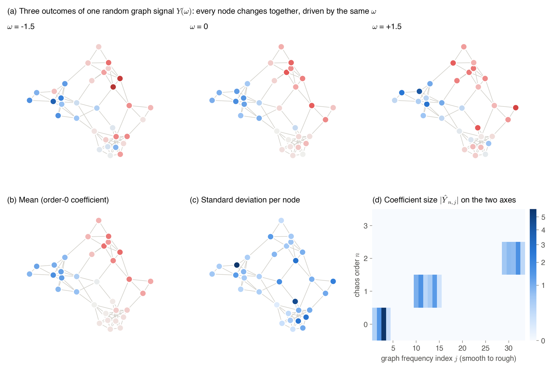
An ordinary, deterministic GNN representation is the special case in which only the coefficients are nonzero. DSS-GNN keeps the first orders and learns how to update them.
The DSS layer
A DSS layer stores, for every node, coefficient vectors , one per chaos order, instead of one hidden vector, and the represented embedding is . The input features are first mapped to these coefficients by learned linear maps, and each layer then updates them along both axes. On the graph axis, every coefficient goes through the low-pass and the high-pass Chebyshev filter, giving and , and on the chaos axis, per-order chaos gates and , which are learned constants or themselves low-order expansions in , weight and combine the two filter outputs.
A neural network also needs a nonlinearity such as ReLU, but the ReLU of a polynomial is not a polynomial, so it mixes the chaos orders and has no closed form. DSS-GNN computes this step by evaluating, applying and projecting back: it evaluates the embedding at fixed values , applies the linear map and the ReLU at each of them, and computes the new coefficients with weights ,
The points and weights are a Gauss–Hermite quadrature rule, and the -point rule computes the Gaussian average of any polynomial of degree up to exactly. The experiments use , which computes the filter and gate terms exactly for , covering the recommended to 2, while at larger these terms are integrated approximately; the ReLU step is always an approximation, and the paper analyzes its error.
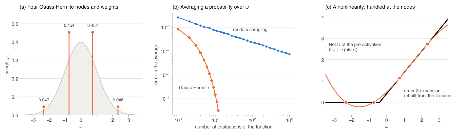
An important consequence is that is never sampled. The network is deterministic from input to output, with no Monte Carlo sampling and no sampling noise in training or at test time, and with , a single coefficient and constant gates, the DSS layer reduces to an ordinary polynomial spectral GNN layer, of which ChebNet and GCN are special cases, so DSS-GNN extends a standard architecture rather than replacing it. The paper’s implementation also offers two variants of the graph-filtering step, described in its appendix, and the variant is selected per dataset on validation data. The cover figure at the top of this post shows the whole architecture.
Reading out uncertainty
After the last layer, a linear map gives each node one logit vector per chaos order, , with one entry per class, and evaluating the expansion at the quadrature points gives logits . Three quantities are read from these coefficients. The first is the predictive distribution, used for prediction and calibration,
which is the class probability averaged over ; the predicted class is the one with the largest , so the prediction and its reported confidence come from the same distribution. The second is the chaos energy, , the total variance of the node’s logits, and training minimizes the cross-entropy of the mean logit plus times the average chaos energy, with chosen per dataset on validation data and zero on three of the 14 datasets. The third, used for OOD detection, is the energy score, computed from the mean logit alone,
where lower energy means more confident. The score comes from energy-based models, in which a classifier’s logits define an unnormalized density over inputs, , whose negative logarithm is the energy, so that inputs unlike the training data, to which the model gives little density, receive high energy. It was proposed for OOD detection on images and adapted to graphs by GNNSafe, which also averages the scores over each node’s neighborhood, a step called score propagation that we follow.
The paper’s Proposition 2 gives two reasons for these choices. The first concerns calibration: when and the loss is smooth, averaging the loss over equals the loss at the mean logit plus a correction, to second order,
where is the covariance of the node’s logits, built from the higher-order coefficients, and is the curvature of the loss. The correction is large only where the logits vary and the loss is curved, which is near a decision boundary, and for cross-entropy it is at most a quarter of the chaos energy, the quantity that the training objective penalizes; on the Minesweeper dataset it concentrates on the hardest nodes. The second concerns OOD detection: if an input lowers every class logit by the same amount, the softmax probabilities do not change, so no score computed from them, such as predictive entropy, can detect the change, while the energy score changes by exactly that amount, and the mean logit therefore keeps information that a softmax discards.
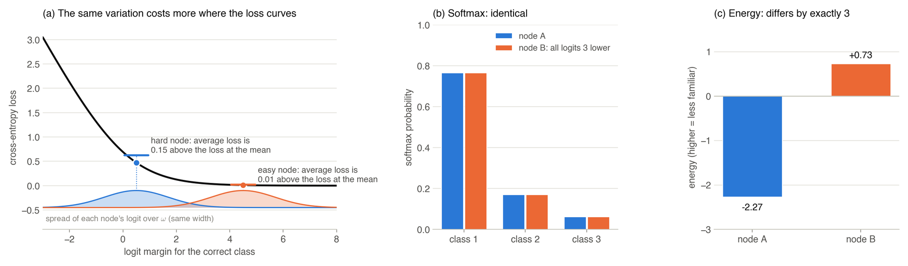
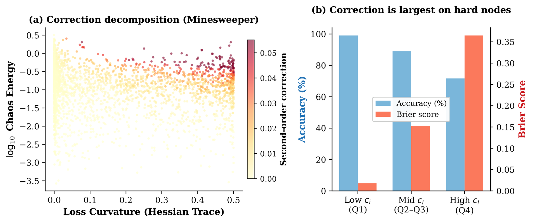
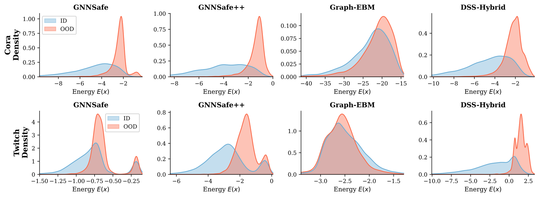
Two further points are needed to state this correctly. The calibration effect comes through training, not through a correction applied at test time: after training, the predictive distribution and the plain softmax of the mean logit agree closely, their predicted classes differing on at most 0.21% of test nodes, and on none at all for 10 of the 14 datasets, and their accuracy and Brier score by at most 0.04 points and 0.003. This holds on the datasets where is zero as well, and no temperature scaling or other post-hoc calibration is used. And because the energy score reads only the mean logit, the design predicts that OOD detection should not depend on the chaos order, which the experiments confirm, since varying only from 0 to 3 leaves the energy AUROC on Cora-structure flat, at 91.0, 91.2, 90.9 and 90.8, in a separate set of runs at one fixed configuration whose level differs from the main results. What the DSS representation adds shows up when everything else is held fixed: on the three Cora settings, with the same energy readout, score propagation and training objective, it separates in-distribution from OOD nodes more widely than the GCN encoder alone does.
Two ways to deploy it
DSS-GNN can be used in two modes, which share the same representation and the same readouts, as the bottom right of the cover figure shows. In the standalone mode the whole network is made of DSS layers. In DSS-Hybrid, a DSS-GNN branch is added next to a conventional encoder, a two-layer GCN in our experiments to match the baselines, and the logits are combined as with a learned scale , the GCN being warmed up for a few epochs before the DSS branch is activated. The chaos-energy penalty keeps the branch from fitting noise in the training distribution, while its two filters can adjust which graph frequencies the model relies on when the distribution changes, a design choice that the experiments support rather than a guarantee.
What the theory says, and what it does not
The paper proves four results. Proposition 1 says that recovers standard spectral GNNs, Proposition 2 explains the readouts, as above, and two theorems describe the layer itself. Theorem 1 concerns its operator structure: without the ReLU, and with a quadrature rule fine enough to be exact, a DSS layer is a linear operator on the joint domain of graph frequency and chaos order, acting frequency by frequency, with the Chebyshev filters setting the response to each graph frequency and the chaos gates setting how the orders mix.
Theorem 2 concerns capacity. If the node features have full rank, which requires at least as many features as nodes, a restricted one-layer DSS-GNN can match the chaos coefficients of any random graph signal driven by a Gaussian variable, up to any chosen order ; as and the width grow, these outputs can approximate any such signal, and for targets that meet a strong smoothness condition, an extension to an entire function, analytic on the whole complex plane, with controlled growth, the truncation error shrinks exponentially in . For the common case of fewer features than nodes, as on Cora with 1,433 features for 2,708 nodes, the same construction matches, through order , every target whose chaos-coefficient columns lie in the span of the features, under one additional positivity condition that can be met by adding a constant feature.
These are statements about what the layer can represent, and they do not by themselves guarantee good calibration, OOD detection or robustness, claims that rest on the experiments below. The exponential truncation bound is consistent with what we observe, since low orders, = 1 or 2, already capture most of the benefit.
Results
We evaluated the standalone model on calibration and DSS-Hybrid on OOD detection and distribution shift, and then cross-evaluated both modes on all three tasks. Calibration was measured on 14 node classification benchmarks, citation, co-purchase, co-authorship, web-page and heterophilous graphs, with 10 splits each, against the uncertainty-aware GNNs TFE-GNN and G-UQ, and with no post-hoc calibration. OOD detection used the GNNSafe benchmark, whose nine node-level settings perturb the graph structure, perturb the features or hold out classes on Cora, Amazon-Photo and Coauthor-CS, and whose two cross-graph settings train on one graph and test on others: on Twitch the German network against the Spanish, French and Russian ones, and on Arxiv papers up to 2015 against papers from 2018 to 2020. The baselines were GNNSafe, GNNSafe++, GPN, Graph-EBM, MC-dropout with 20 passes and Deep Ensembles of 5 models, and DSS-Hybrid follows the GNNSafe++ protocol, with the same GCN configuration, the same energy-margin training objective and the same score propagation, so that the two differ only in the DSS branch. Distribution shift was measured on 7 concept-shift settings of the GOOD benchmark against 13 baselines, most of them designed for distribution shift, such as IRM, VREx, GroupDRO and TAR, while DSS-Hybrid is trained with plain empirical risk minimization.
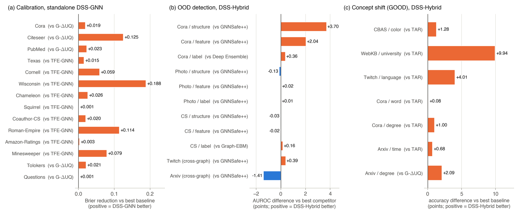
Standalone DSS-GNN has the lowest Brier score among the compared uncertainty-aware methods on all 14 datasets and the best accuracy on 13, the exception being Squirrel, where TFE-GNN is more accurate, at 71.56% against 68.06%. The margins vary, large on Wisconsin, Minesweeper, Citeseer and Roman-Empire and 0.003 or less on Squirrel, Amazon-Ratings and Questions, and the gains are not an accuracy effect, since standard GNNs such as GCN and GAT match or exceed DSS-GNN’s accuracy on Cora and Citeseer but are less calibrated. With , that is, with no chaos terms, DSS-GNN is still a competitive two-filter spectral GNN, so the comparison across isolates what the chaos expansion adds.
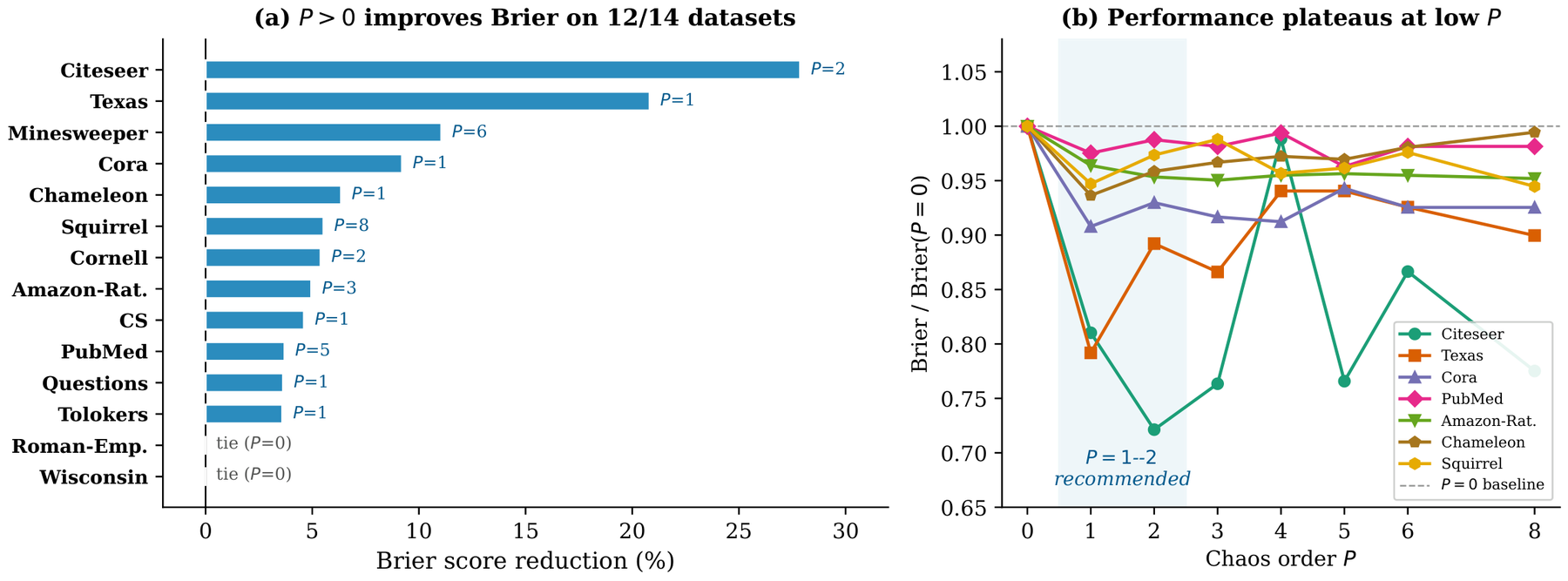
Raising above 0 improves the Brier score on 12 of the 14 datasets, and on every dataset or is within 0.02 of the best order tried, so we recommend to 2 as the default. is exactly a Gaussian representation, and the higher orders add non-Gaussian structure that matters on some datasets: on Citeseer, going from to lowers the Brier score from 0.346 to 0.308.
For OOD detection, DSS-Hybrid has the best AUROC on 6 of the 9 node-level settings, including all three Cora settings, at 94.32, 97.60 and 94.11 against 90.62, 95.56 and 92.75 for GNNSafe++, and on the other three it is within 0.13 points of the best method, where both it and GNNSafe++ are above 99.6. On Twitch it improves on GNNSafe++ in every metric, with an AUROC of 95.75 against 95.36 and a false positive rate at 95% recall of 22.40 against 33.57, while on Arxiv it is 1.41 AUROC points behind GNNSafe++, at 73.36 against 74.77, though it has the best false positive rate and in-distribution accuracy. Against MC-dropout and Deep Ensembles, which receive the same score propagation, DSS-Hybrid has the higher AUROC on all 11 settings, in one forward pass against their 20 passes and 5 models, and score propagation itself contributes up to 18.2 AUROC points, on Twitch.
Under distribution shift, DSS-Hybrid trained with plain empirical risk minimization has the highest mean shifted accuracy on all 7 GOOD concept-shift settings, by margins from 0.08 points on GOOD-Cora/word to 9.94 points on GOOD-WebKB/university. The chaos terms contribute here too, since in the standalone model improves shifted accuracy over on GOOD-Cora/word by 1.7 points, on GOOD-Cora/degree by 1.2 and on GOOD-Arxiv/time by 0.6.
We also ran each mode on the other’s tasks. On calibration, the standalone model has the best Brier score on all 14 datasets and is stronger than the hybrid on 13 of them, Tolokers being the exception, while the hybrid is never worse than its own GCN base beyond noise and gains a great deal where the GCN is weak, as on Roman-Empire, with 27.7 points more accuracy and a Brier score lower by 0.33. On OOD detection, the standalone model is effective on 10 of the 11 settings, its energy score failing to separate the groups only on Twitch, and the hybrid is stronger than the standalone on 10 of the 11. On concept shift, the standalone model is above every published baseline on 5 of the 7 settings and at the level of plain empirical risk minimization on the other 2, while the hybrid is highest on all 7. This gives practical guidance: the standalone model is the choice when calibration on a single graph matters most, especially when neighbors tend to differ, and the hybrid is the choice when a strong conventional encoder already exists, for transfer across graphs, and for OOD detection with few labels.
The cost is moderate. Graph filtering and coefficient memory grow with the number of chaos orders , and the nonlinearity step with the number of quadrature points , but no eigendecomposition is ever computed, and the measured training time per epoch at is 2.9 times that of on Cora, 1.2 times on Amazon-Ratings and 1.1 times on ogbn-arxiv, where each additional order adds about 4%, while memory grows linearly with .
Limitations
The two modes share a representation and readouts but are not interchangeable everywhere. The standalone model needs BatchNorm to train stably when labels are scarce, as every baseline encoder in the OOD benchmark does, and its energy score fails on Twitch, while the hybrid inherits the limits of its encoder, so that on small heterophilous graphs, where a GCN is a poor fit, it matches its GCN base but does not improve on it. All variation comes from a single Gaussian shared by every node, so variations at different nodes are perfectly dependent and the model cannot represent independent noise at each node; this is enough for per-node calibration and OOD scores, and it is what makes single-pass quadrature possible, but joint uncertainty across nodes is not modeled, and with latent variables a full quadrature grid would need points, a cost that sparse grids can reduce and that we leave to future work. The expansion also adds the compute overhead reported above, and the theorems describe what the layer can represent, while the benefits at the level of tasks are established empirically, on the benchmarks we tested.
Takeaways
Uncertainty can be part of the representation itself: writing each node’s embedding as a polynomial in one Gaussian variable gives every node a mean, in order 0, and a description of its variation, in the higher orders, which the network learns directly. Graph frequency describes how a pattern varies across the network and chaos order how it varies with the random variable, both coming from orthonormal eigenbases, and the DSS layer filters along both. Gauss–Hermite quadrature replaces random draws, so one deterministic forward pass gives all the uncertainty readouts, and one representation serves several tasks through matched readouts, the averaged predictive distribution serving prediction and calibration, the mean-logit energy serving OOD detection, and a regularized DSS branch beside a standard encoder helping under distribution shift. If you work with graphs where decisions depend on knowing how much to trust a prediction, we hope DSS-GNN is useful to you, and the code is on GitHub.
This work was partially supported by NSF 2303037, NSF 2312501, NSF 2531008, NSF 2553619, SRC JUMP 2.0 Center, CDSC Industry Partners, Amazon Research Awards, Snapchat, and Google Gifts. Part of this work was done while Fred Xu was an intern at Block, Inc., and we thank Block, Inc. for its support. The cover figure and the figures of the second-order correction, the chaos order and the energy densities are from the paper; the other figures were made for this post, with synthetic examples except for the results chart, which uses the numbers in the paper’s tables.