AIResearchGraphsAnomaly Detection
Graph Anomaly Detection as Finite-Horizon Control
EB-GAD scores graph anomalies with no labels and no training: empirical Bayes fits a graph-aware Gaussian model of normal in closed form, and each node is scored by the finite-horizon control energy needed to steer a neutral start to it under a graph Ornstein–Uhlenbeck process. Best or tied-best AUROC on 9 of 11 benchmarks.
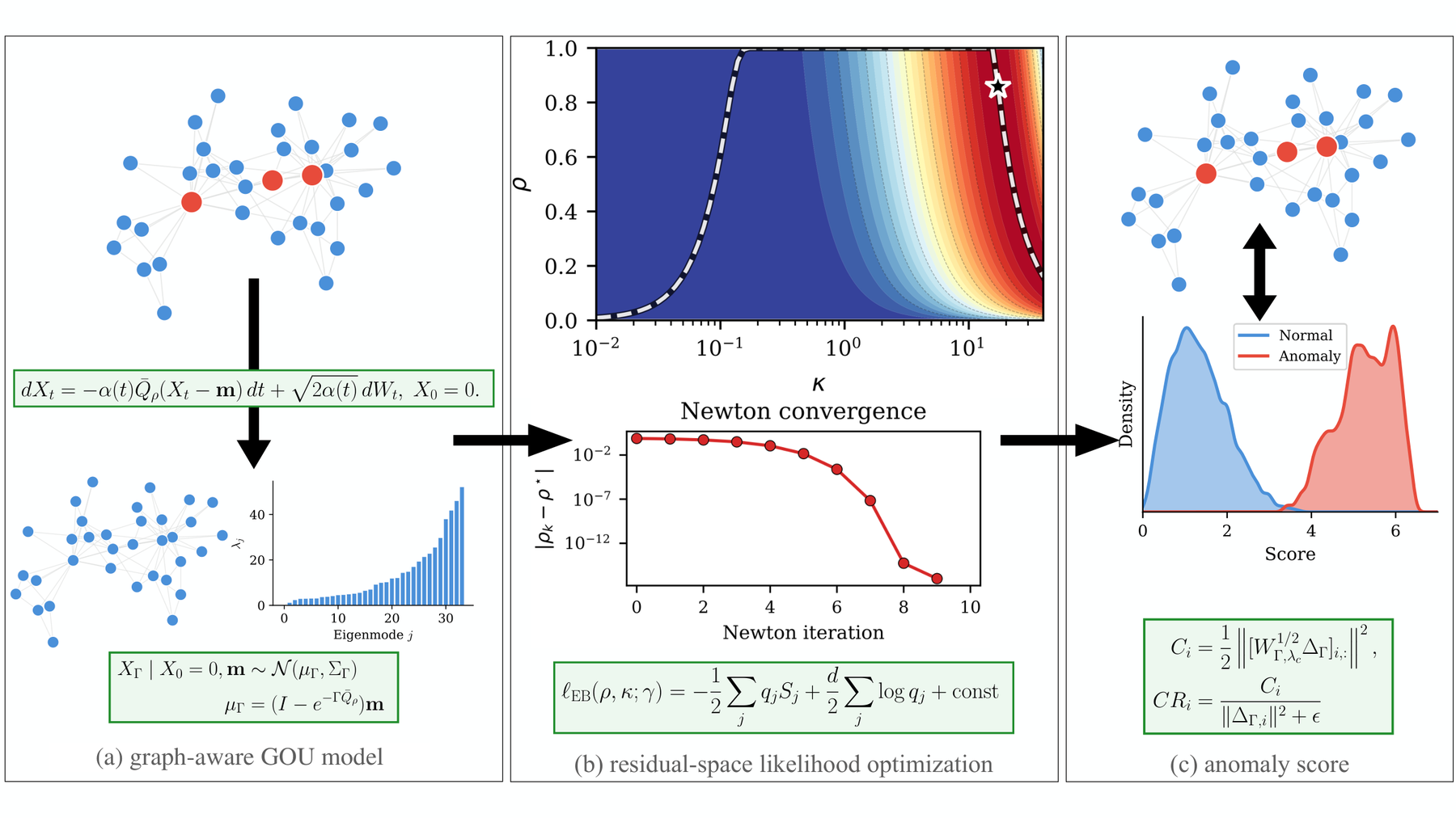
This post is a tour of our NeurIPS 2026 paper, “Graph Anomaly Detection as Finite-Horizon Control: Training-Free Scoring via Empirical Bayes,” written with Thomas Markovich of Block, Florence Regol of Mila and Yizhou Sun of UCLA. Its aim is to find the unusual nodes in a network, such as fraudulent accounts, fake reviewers or suspicious transactions, without labels and without training a neural network. We write down an explicit statistical picture of what “normal” looks like on a graph, let the unlabeled data fit its three knobs, and score each node by how much effort it takes to steer a neutral starting point to that node under a simple graph-aware dynamics. On 11 benchmarks the method, which we call EB-GAD, has the best or tied-best AUROC on 9, with its largest margins on financial fraud networks of up to 3.7 million nodes.
Why anomalies in networks are hard
Many of the systems we care about are networks, in which a payment platform connects accounts by transactions, a review site connects users to products, and a social platform connects people to people. Each node, an account or a user, comes with features such as transaction sizes, account age or statistics of its review text, while the edges say who interacts with whom, and graph anomaly detection asks which nodes look abnormal. Two things make the question hard in practice.
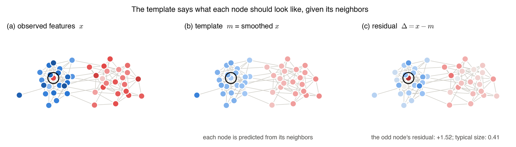
The first difficulty is that there are almost no labels, because fraud is rare, confirmed cases are scarce and arrive late, and fraudsters change their tactics, so we want an unsupervised method, one that gives every node a suspicion score using only the network itself. The second is that context matters, since a node can look perfectly ordinary on its own and still be odd for where it sits in the network, as the toy example below shows.
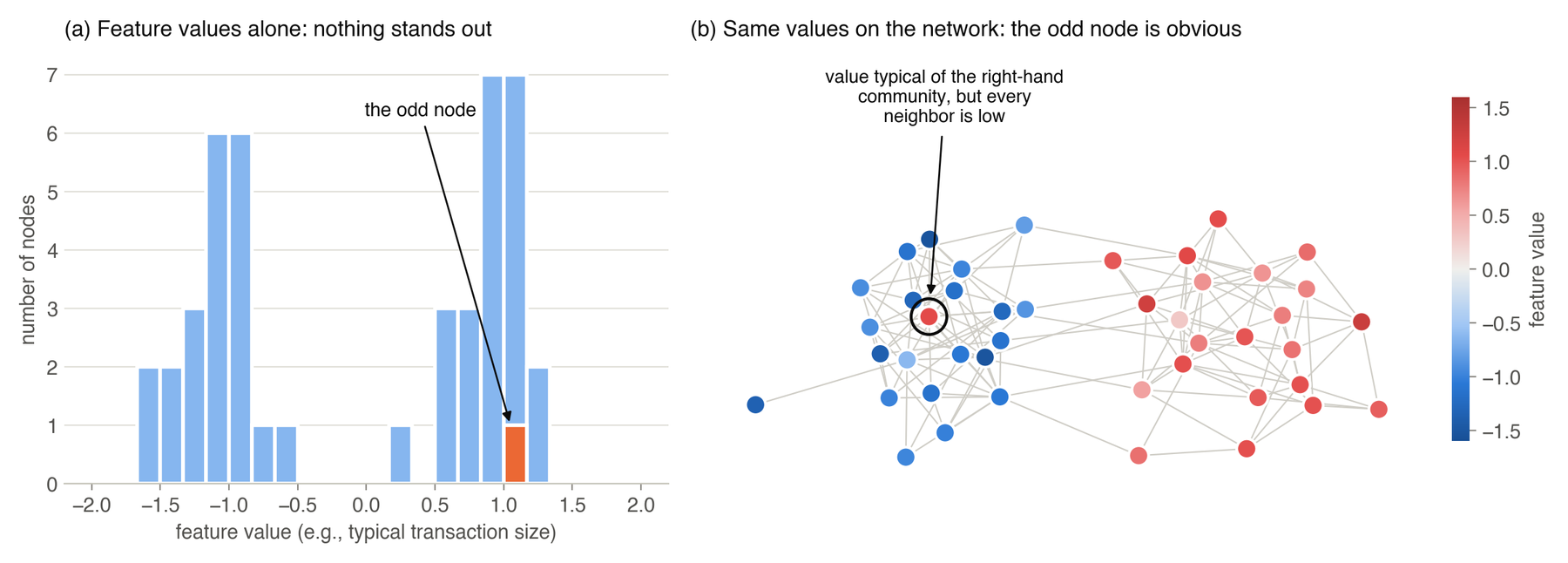
A detector therefore has to decide how much the network should define what counts as normal. In some networks the edges connect similar nodes and are a reliable guide, but in fraud they can mislead, since fraudsters deliberately connect to ordinary accounts in order to blend in, and we call this question graph trust. Most existing methods answer it implicitly, through the design of a neural network, a training loss that reconstructs the graph or contrasts views of it, and a sweep of hyperparameters, and the resulting scores are expensive to obtain, hard to interpret and unstable from one network to the next. In our benchmark several published methods even score below chance on some datasets. Our goal was the opposite: to make every choice explicit, to fit it from unlabeled data in closed form, and to train nothing.
An anomaly is a surprise
A classic way to define an anomaly score is surprise, which means building a model of normal data and scoring a point by how unlikely it is,
If the model of normal is a Gaussian with mean and covariance , surprise becomes a weighted squared distance, the Mahalanobis distance,
The matrix is called the precision, and a useful way to read it is as a price list for deviations: moving in a direction where normal data varies a lot is cheap, while moving against the grain of the data is expensive.
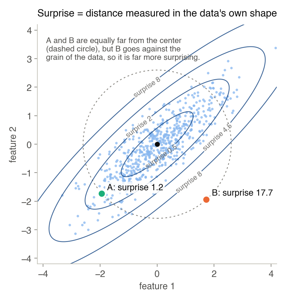
The whole game therefore comes down to two choices, what normal looks like, which is the mean, and which deviations are cheap or expensive, which is the precision, and EB-GAD builds both from the graph.
Patterns on a graph have frequencies
To use the graph, we need a way to say whether a pattern of values over the nodes is smooth, with neighbors agreeing, or rough, with neighbors disagreeing. The tool is the graph Laplacian , where is the adjacency matrix and holds the node degrees, and for a pattern that assigns one number to each node,
which is small when connected nodes have similar values and large when they do not. In practice EB-GAD uses the symmetric-normalized Laplacian , whose eigenvalues lie between 0 and 2, so that high-degree nodes do not dominate, but the intuition is the same. The eigenvectors of play the role of frequencies on the graph, as sines and cosines do for sound: each eigenvector is a pattern over the nodes, and its eigenvalue measures how rough that pattern is, so that a small means a smooth, slowly varying pattern and a large one a pattern that flips sign across many edges.
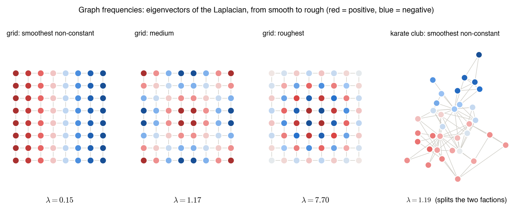
Any feature pattern can be written as a mix of these modes, and we write for how much energy a pattern puts into mode , which lets us speak of the smooth and the rough parts of the data, exactly what a model of normal on a graph needs.
EB-GAD’s picture of normal
EB-GAD’s model of normal has two ingredients, a template, which says what each node should look like, and a precision, which says how much each kind of deviation costs, and three interpretable knobs control them.
The template
The template is a smoothed version of the features,
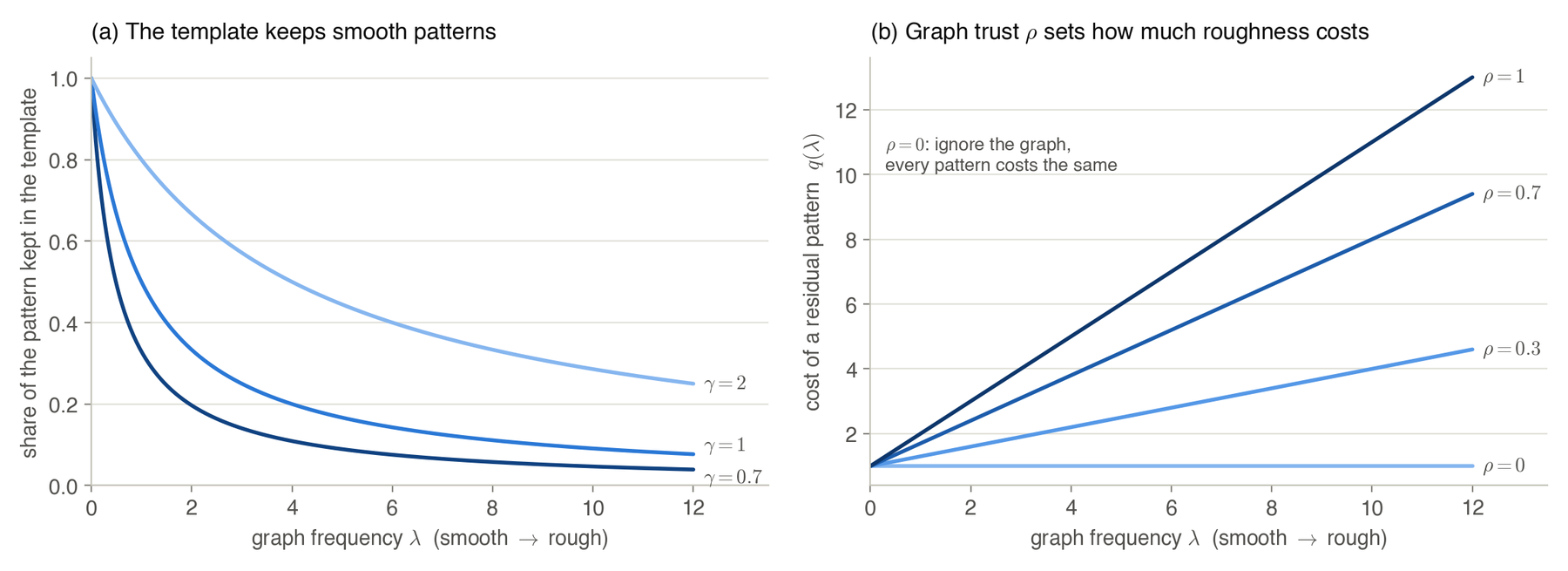
which in frequency terms multiplies mode by , keeping smooth patterns and filtering out rough ones, with the bandwidth setting how aggressive the smoothing is. It is the graph version of ridge or Tikhonov smoothing, since up to a constant factor it is the pattern that stays closest to while paying a penalty for roughness, and each node’s template value is, in effect, a prediction from its neighborhood, and what we actually score is the residual, the part of each node that its neighborhood does not explain,
The precision
Next we need a price list for residuals, and EB-GAD uses
which charges each mode the price
Both knobs have plain meanings, for graph trust , a number between 0 and 1, decides how much the graph counts: at the graph is ignored and every residual pattern costs the same, while at rough residual patterns, in which neighbors disagree, are much more expensive than smooth ones. The length-scale sets the frequency below which all patterns cost about the same and above which the cost grows with roughness. The form is borrowed from Matérn Gaussian processes on graphs, whose precision is the graph counterpart of the Matérn family that machine learning uses for smooth functions in space; EB-GAD takes , which keeps as sparse as the graph itself, a Gaussian Markov random field, and mixes it with the identity through , so that a single number moves the model from ignoring the graph to trusting it fully and the data can choose the point on that path.
With the template and the precision in place, the simplest anomaly score is each node’s share of the Gaussian surprise of the residual,
When nodes have many features, each feature column is treated as its own signal on the graph, all of them sharing the same . This equilibrium score is EB-GAD’s starting point, and the reason for its name, and for going beyond it, will become clear once we add time.
Empirical Bayes: letting the unlabeled data set the knobs
We now have three knobs, graph trust , length-scale and template bandwidth , and the question is where their values come from when there are no labels. Empirical Bayes is the classical answer to exactly this situation, in which many units share a few unknown parameters of a prior and nothing outside the data fixes them. A fully Bayesian analysis would put a further prior on those parameters, whereas empirical Bayes estimates them from the data themselves, by maximizing the marginal likelihood, the probability of the observations once the latent quantities have been integrated out. Herbert Robbins introduced the approach in the 1950s, Bradley Efron and Carl Morris showed in the 1970s that it explains the power of the James–Stein estimator, which shrinks many means toward a common value and beats estimating each of them separately, and machine learning knows it as type-II maximum likelihood or evidence maximization, the standard way of fitting the hyperparameters of a Gaussian process.
It suits graph anomaly detection for two reasons, the first being that every node is a unit and all of them share the same three knobs, so thousands or millions of nodes inform three numbers and the fit is stable even though no single node says much, and the second that the quantity being maximized is the probability of the whole unlabeled graph, which is dominated by normal nodes because anomalies are rare. In EB-GAD the latent quantity is the residual field: each feature column of the residual is modeled as , independently across the features, so its log-likelihood is a sum of quadratic forms and log-determinants . In the eigenbasis of the Laplacian both separate by mode, the quadratic forms into times the residual energy and the log-determinant into , and because everything is linear and Gaussian the whole likelihood has a closed form,
where the constant does not depend on the knobs. The two terms pull in opposite directions, since the second rewards high precision, a confident and concentrated model, while the first penalizes high precision wherever the data actually has energy, and the balance between them is a built-in Occam’s razor, in which the fitted price list is as strict as the data allows.
Because the likelihood is dominated by normal nodes, the fitted model approximately describes normal behavior even though no label is used. In our robustness study, contaminating a dataset with up to 24% anomalies barely moved the fit, and detection of the original anomalies dropped by 1.1 AUROC points on Weibo. The fit itself is cheap, a few Newton steps for , in which the likelihood is concave, and small grids for and .
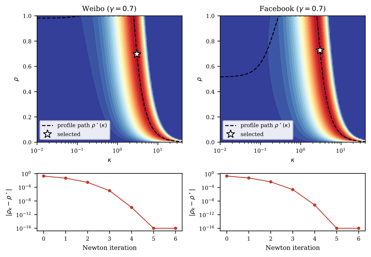
This is what we mean by training-free: no neural network, no gradient descent, no epochs, no labels and no validation set. EB-GAD does fit three numbers, by maximizing a closed-form likelihood on the unlabeled graph, so “training-free” does not mean “hyperparameter-free.”
Adding time: normal data as a relaxation process
So far the model is static, a Gaussian with mean and precision , and the equilibrium score weighs each graph mode by its stationary variance and nothing else. Any other weighting of the modes would be an ad hoc spectral filter with no tie to the fitted model, so the key idea of the paper is to view the Gaussian as the end point of a simple process, because that process gives a whole family of weightings, all derived from the same model. Picture a ball attached by a spring to the template and jiggled by random noise: started anywhere, it drifts toward the template and then keeps jiggling around it. This is an Ornstein–Uhlenbeck process, and our graph-aware version is
where is a Brownian motion. Leonard Ornstein and George Uhlenbeck introduced the process in 1930 as a model of the velocity of a Brownian particle slowed by friction, and it has a special place among random processes, since by a theorem of Doob it is, up to rescaling, the only process that is at once stationary, Gaussian and Markov. It is also the Langevin diffusion of a Gaussian: for any energy the dynamics settle into the distribution proportional to , and when is the quadratic surprise , its gradient is linear and the Langevin diffusion is exactly the process above. Readers who work on generative models will recognize it as the forward process of score-based diffusion models, which relaxes data toward white noise; here the process starts from a neutral point and relaxes toward the fitted graph Gaussian instead.
These properties are what make the formulation natural rather than decorative, for the process is the canonical dynamics whose resting state is our fitted Gaussian, and its drift is the fitted precision itself, so no new parameter is needed to describe it; it is linear, so every quantity we need has a closed form in the Laplacian’s eigenbasis; and it relaxes each mode at its own rate, so time becomes a principled knob for weighting smooth against rough deviations. The paper writes the process with a rate that may vary in time, as in the cover figure, but only the integrated horizon matters for the scores, so we keep the rate constant here. Run long enough, the process settles into exactly our Gaussian , but before it settles something interesting happens, for each graph mode relaxes at its own speed : rough modes, with large , settle almost at once, while smooth modes take their time.
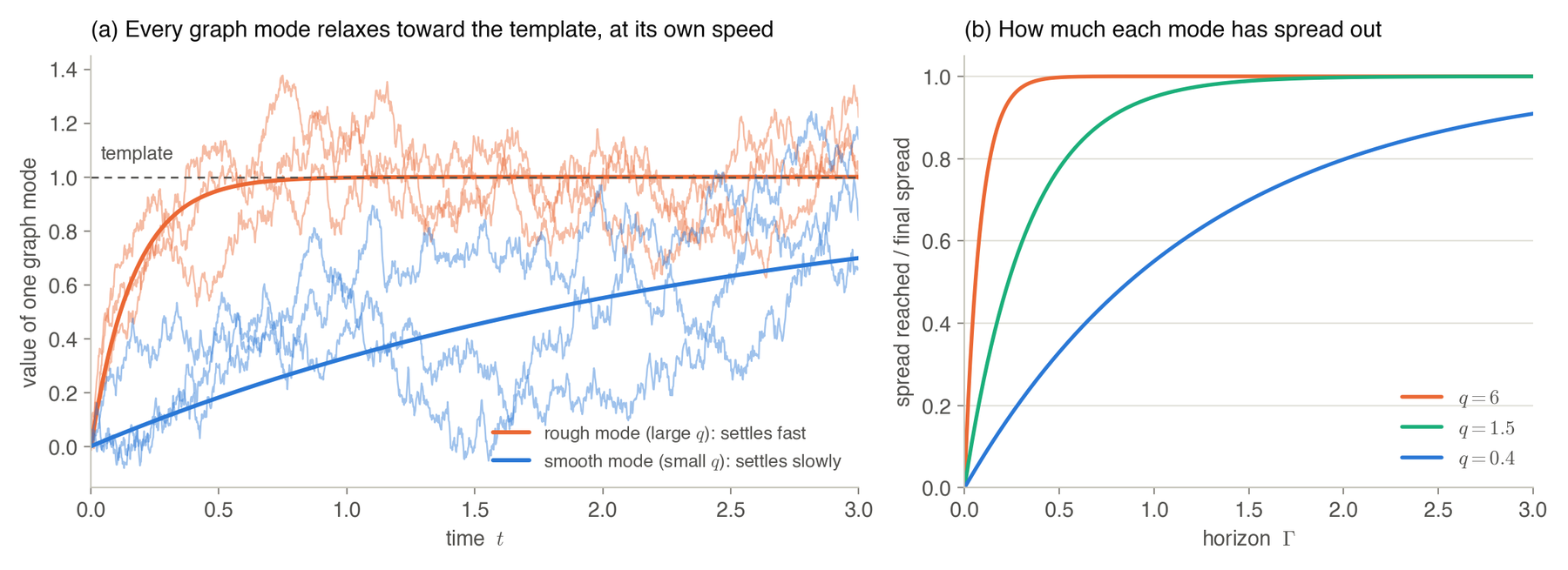
Started from a neutral point , which means “average” because the features are standardized, the state after a time horizon is Gaussian, with
the second being the spread of mode . We do not claim that real fraud data evolved by this process, for the dynamics are a modeling device: they are the canonical process whose resting state is the Gaussian we fitted, so every score derived from them shares the same fitted model of normal.
The score: how hard is it to steer to this node?
Now imagine that we could push the process with a steering input , and ask what is the least total effort needed to start at the neutral point and land exactly on the observed node at time . For a normal node the process drifts there almost by itself, while for an anomaly we have to push hard, and for this linear system the minimum steering energy has a closed form, which equals the surprise of the observation under the time- Gaussian,
The equality between effort and surprise is a classical fact of linear control theory rather than a coincidence. For a linear system , the least energy needed to move between two states in time is a quadratic form in the inverse of the controllability Gramian , a result that goes back to Kalman, and for our process, with and , this Gramian is exactly the covariance of the noise-driven state. The cheapest way to reach a point and the probability of reaching it by chance are two readings of the same matrix, so the score has both a statistical meaning, surprise under the fitted model, and a mechanical one, how hard the graph dynamics resist arriving at this node.
We call this the finite-horizon control energy, and on mode the cost per unit of residual is
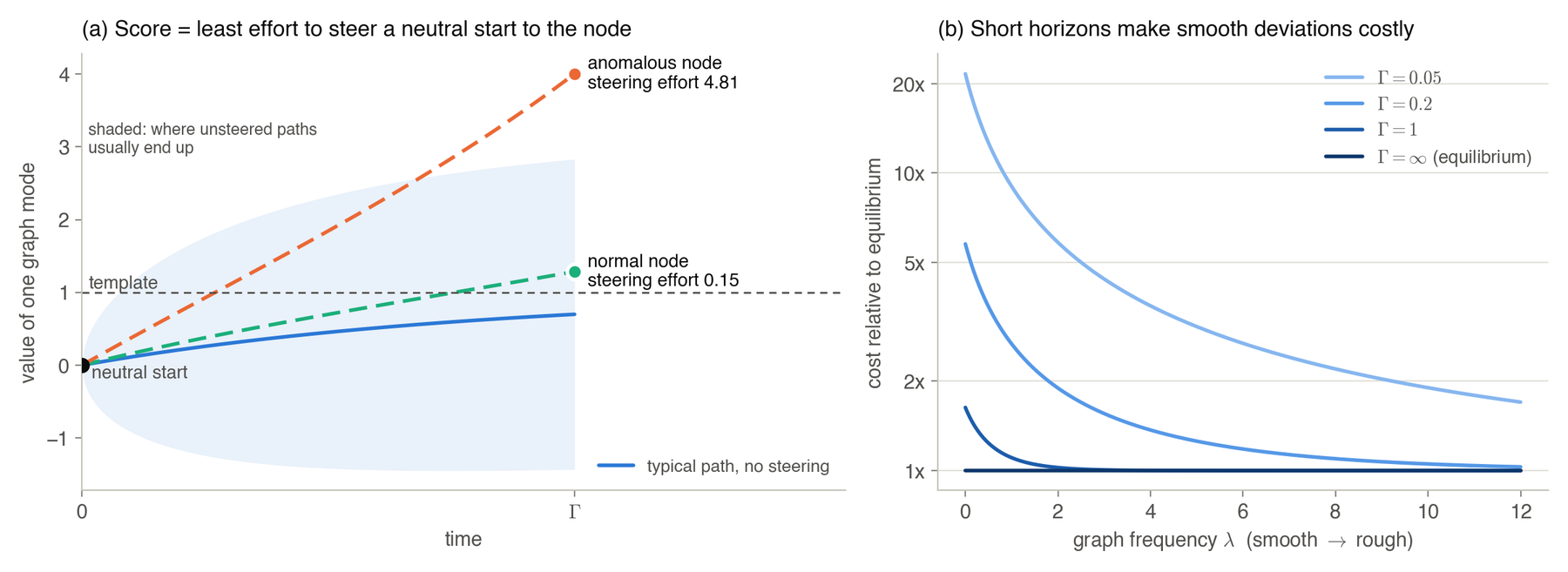
The right-hand panel is the heart of the idea, for at a long horizon every mode has settled and the score is the equilibrium surprise , but at a short horizon the smooth modes have not had time to wander, so that any deviation in a smooth direction is expensive. A short horizon therefore asks a different question, whether a node is surprising before its neighborhood’s pattern has fully settled, and since different networks reveal their anomalies at different horizons, we keep the whole range.
Two more dials complete the family, the first of which is an endpoint tolerance that allows a little slack instead of landing exactly on the node, so that the per-mode cost becomes and the score checks whether the evidence survives softer matching. The second is a ratio score, needed because some normal nodes simply have large residuals overall: dividing a node’s control energy by the size of its residual, , asks a scale-free question, how much of this node’s deviation is of the kind the graph says is expensive.
A bank of scores, and choosing one without labels
Sweeping the horizon and the tolerance gives a bank of scores, all of which share one fitted model of normal, so that they are comparable and calibrated against the same baseline. EB-GAD uses them through four families. The equilibrium anchor, or its ratio, is the classic Gaussian surprise of the residual and the default whenever the finite-horizon diagnostics are not stable enough to justify leaving it; the control energy measures the absolute effort to reach a node at a finite horizon and is used when the size of the residual is itself informative; the control ratio measures the share of the residual that the graph makes expensive and is used when raw residual size would otherwise dominate; and profile aggregation combines the evidence across horizons and tolerances when the signal is spread over many of them.
For a new network, with no labels, EB-GAD chooses among these with a fixed, label-free selector that is the same on every dataset. Simple graph statistics pick the family, namely how similar the features of connected nodes are, which is feature homophily, how dense the graph is, and how many features each node has, and within the family the selector prefers a score that departs clearly from the fitted model of normal and whose ranking stays stable when the horizon or the tolerance is nudged, favoring robust scores over one lucky configuration. The selector’s cutoffs are engineering defaults developed on these benchmarks rather than derived from a single principle, but they are robust, since perturbing each of its 21 cutoffs by ±25% leaves the selection unchanged in 99.4% of cases. The figure at the top of this post shows the whole pipeline, from the graph-aware process around the template, through the empirical-Bayes fit of the precision, to the bank of scores and the selector.
A worked example: the karate club
Zachary’s karate club is a classic social network of 34 members, recorded just before the club split in two. As features we use each member’s connection profile, the row of the adjacency matrix, and we run the paper’s pipeline as it is.
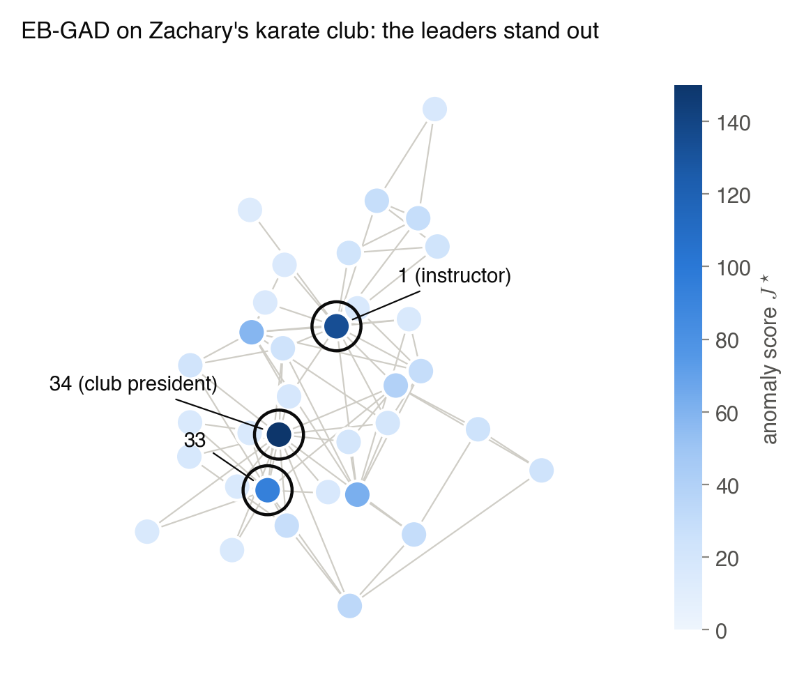
The leaders stand out, as they should, since their connection profiles are unlike anyone else’s, and the fitted knobs are interpretable: empirical Bayes sets graph trust to , because when the features are the connections themselves, the graph’s information is already in the template, and the fit correctly declines to count it a second time in the precision. Zachary’s published data is also inconsistent about one edge, between members 23 and 34, and toggling it changes the scores only locally, with 98.8% of the change falling on the two endpoints and their neighbors, while the overall ranking barely moves, at a rank correlation of 0.989.
Results
We compared EB-GAD with 9 baselines on 11 benchmarks, 7 standard anomaly-detection graphs drawn from social, review and citation networks and 4 financial fraud networks with up to 3.7 million nodes. EB-GAD runs with one fixed procedure everywhere, and no label enters any step before evaluation.
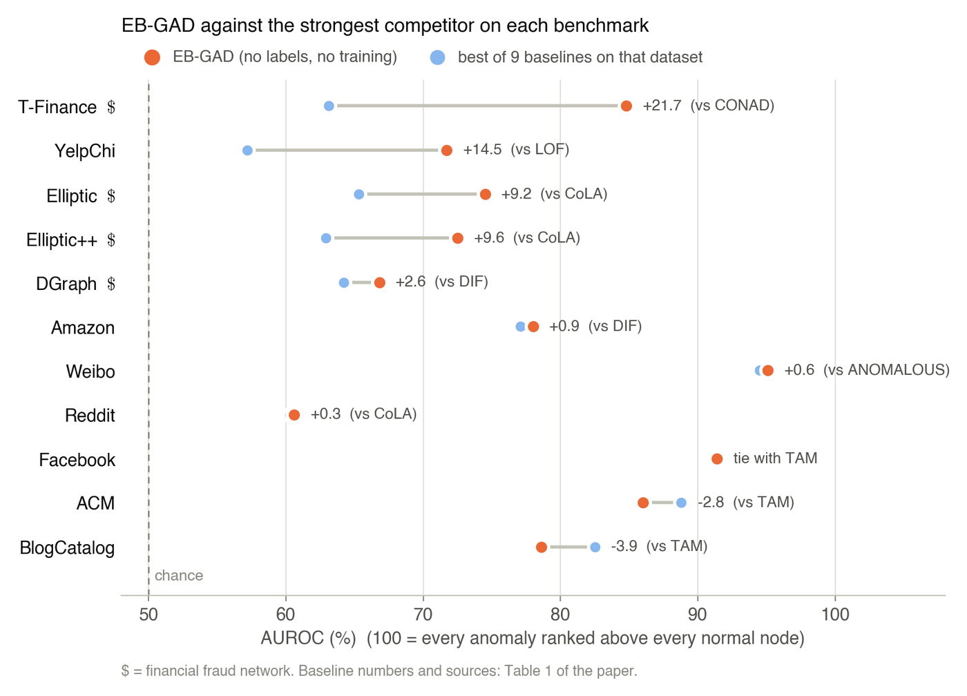
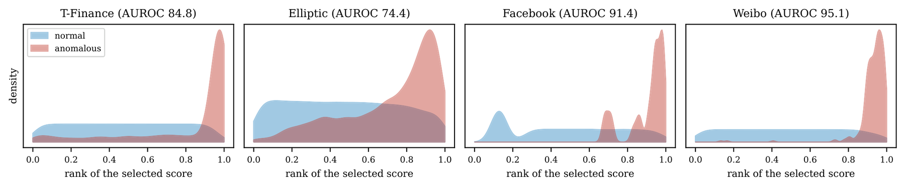
EB-GAD has the best or tied-best AUROC on 9 of the 11 datasets, with large margins on financial fraud, 21.7 points on T-Finance, 9.2 on Elliptic, 9.6 on Elliptic++ and 2.6 on DGraph, and 14.5 points on the YelpChi review-fraud graph. It is second on BlogCatalog and ACM, behind TAM, a strong method built on local neighbor affinity, and on several datasets its scores separate the two groups cleanly.
The time dimension earns its place: holding the fitted model fixed, the finite-horizon families improve on the equilibrium score by 3.6 points on Facebook, 4.7 on T-Finance and 4.7 on ACM, and are at parity elsewhere, a gain that comes from aggregating and normalizing a family of scores that share one fitted model rather than from one lucky horizon. The method is also fast, for on 16 CPU threads a full run takes from 8 seconds on Facebook to 33 minutes on DGraph, with its 3.7 million nodes, 30 minutes of which go to computing the graph’s smoothest modes, while the two trained graph baselines that fit in memory on DGraph need 65 and 69 minutes on a GPU.
Limitations
The method has limits, which the paper reports in full, and the first is that one selection rule was chosen after seeing results. The Weibo and Reddit numbers depend on how the bandwidth of the equilibrium anchor is chosen, and we adopted the current rule after evaluating the first one, under which these two datasets score 92.5 and 48.5 and the count falls to 7 of 11; the paper reports both. The model is also Gaussian, and while heavy-tailed residuals cost at most 0.7 points in a controlled test, a normal population made of two distinct groups costs 9 to 19 points, and binary (0/1) features fall outside the model altogether. Heterophilic graphs remain hard, for on BlogCatalog and ACM EB-GAD trails TAM, and alternative templates did not close the gap. Finally, on networks of users the scores can encode biases of degree or activity, since very active or very connected users may look unusual, so they should be audited across groups of users before they are used for real decisions.
Takeaways
What is usually hidden inside a neural architecture can be written down explicitly, as a template, which says what a node’s neighborhood predicts, and a precision, which says what deviations cost, with knobs whose meanings are plain. Because anomalies are rare, empirical Bayes can set those knobs from unlabeled data and recover a model of normal behavior in closed form, with no training at all, and viewing the fitted Gaussian as the resting state of a relaxation process turns anomaly scoring into a question of steering effort, which yields a whole bank of scores that share the same fitted model and from which simple graph statistics and a preference for stable scores choose, conservatively and without labels. If you work with networks where labels are scarce and decisions need to be explained, we hope EB-GAD is a useful and transparent starting point, and the code is on GitHub.
We thank Block for supporting this work, part of which was carried out while Fred Xu was an intern at Block. This work was partially supported by NSF 2303037, NSF 2312501, NSF 2531008, NSF 2553619, SRC JUMP 2.0 Center, CDSC Industry Partners, Amazon Research Awards, Snapchat, and Google Gifts. The cover figure, the likelihood landscape and the score densities are from the paper; the other figures were made for this post, and the karate-club scores come from the paper’s own pipeline.