AIResearchGenerative ModelsOptimal Transport
Improving Function Space Flow Matching with Kernel Optimal Transport
kFFM replaces the random noise–data pairing of Functional Flow Matching with entropic optimal transport under a kernel-induced cost, the coupling behind the Hilbert Sinkhorn Divergence: a signature kernel for paths, a Sobolev or Euclidean RBF for fields. Same network, same loss, 5–7% more training time, and better samples on eight time-series and PDE benchmarks.
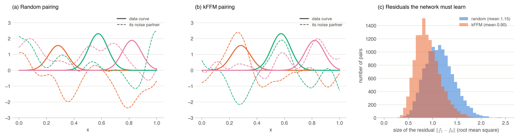
This post introduces our NeurIPS 2026 paper, “Improving Function Space Flow Matching with Kernel Optimal Transport,” written with Thomas Markovich of Block, Barbora Barancikova of Imperial College London and Yizhou Sun of UCLA. Many scientific datasets are made of functions, such as temperature curves, gene-activity time series, volatility paths and snapshots of a fluid. Functional Flow Matching (FFM) learns to generate such data by gradually turning random functions, the noise, into realistic ones, but during training it pairs each noise sample with a data sample at random. Our method, kernel Functional Flow Matching (kFFM), pairs each noise sample with a data sample that already resembles it, by solving a small optimal-transport problem in every training batch under a notion of distance designed for functions: a signature kernel for paths, and an RBF kernel on a derivative-aware Sobolev norm for fields. Nothing else changes, neither the neural network nor the training loss, and training takes 5–7% longer at the largest resolution we train. We prove that this kernel pairing is well-posed and bounded on general function spaces, split its gap to standard optimal transport into interpretable terms, and show that it is stable as the grid is refined. On eight time-series and PDE benchmarks, kFFM has the lowest MMD of all compared methods on every dataset and beats FFM with seed-paired significance on all eight (on three of them while also using a different noise distribution), and the gains hold under non-kernel metrics and on a turbulent Navier–Stokes benchmark.
Why generate functions?
Some data are best thought of as functions rather than as lists of numbers. A weather station’s average temperature over the year is a curve, and so is the activity of a gene over time, or a country’s population from 1950 to 2018; the variance of a stock in a stochastic volatility model traces a rough, jagged path; and the vorticity of a two-dimensional fluid is a field, one number at every point of a square.
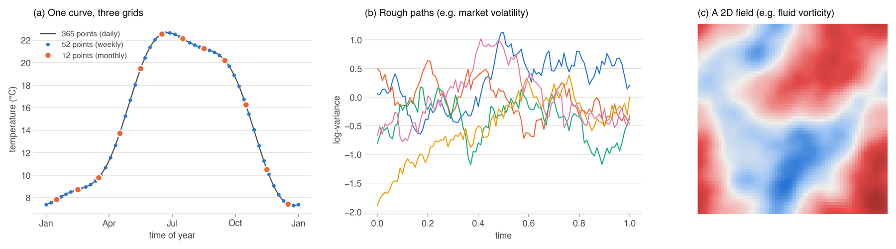
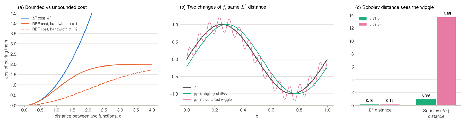
A generative model for such data learns their distribution and can then produce new, realistic samples, such as plausible temperature profiles, volatility scenarios or fluid states, and two properties make this setting different from generating images or vectors. The first is that the grid is not the object: the left panel above shows one curve at three resolutions, and a good model should learn the curve rather than the grid, so that it can be trained at one resolution and sampled at another. The second is that geometry matters, since two functions can be close or far apart in ways a flat list of grid values does not capture, one being a slightly shifted copy of the other, or the same shape with fast wiggles on top, or a path with the same overall trend but a very different roughness.
Our paper improves one step of a strong existing method for this problem, and it draws on more mathematics than most machine-learning papers: function spaces, probability measures on them, optimal transport, kernels and path signatures. The first half of this post builds these up one at a time, each with pictures, and the second half uses them to explain kFFM, its theory and its results. Readers who already know a topic can skip its section, and the method itself is summarized in the section “kFFM on one page.”
Functions as points in a space
To do geometry and probability with functions, we treat each function as a single point in a space. Functions can be added and scaled pointwise, so they form a vector space, but an infinite-dimensional one, and the workhorse is , the square-integrable functions on a domain , with inner product and norm
A Hilbert space is an inner-product space that is complete, meaning that sequences whose terms get arbitrarily close to each other converge to an element of the space. Like , a Hilbert space has orthonormal bases: on a periodic interval the Fourier modes are one, and every function is the sum of its Fourier series,
so that a function is an infinite sequence of coefficients, an “infinite-dimensional vector.”
A computer stores finitely many numbers, grid values or, equivalently, the first few Fourier coefficients, so discretization is projection: keeping the modes up to is the orthogonal projection onto a finite-dimensional subspace . Both the neural operator and the Sinkhorn solver in kFFM work with such truncated representations, so we will need to know how much is lost.
Sobolev spaces measure smoothness. Differentiating multiplies the -th Fourier coefficient by , so a function with square-integrable derivatives has coefficients that decay fast enough for
to be finite; this norm is equivalent, up to constants, to . The functions for which it is finite form the Sobolev space , with and a larger meaning smoother functions, and solutions of PDEs naturally live in Sobolev spaces. Smoothness and decay go together, for a jump gives coefficients of size , a kink , and an analytic function decays exponentially.
This tells us how much discretization loses. For a function in and a weaker norm with , one line of algebra bounds the truncation error,
so that the smoother the function relative to the norm we measure in, the faster the error vanishes. This inequality is the engine of our discretization theorem, which we will meet later.
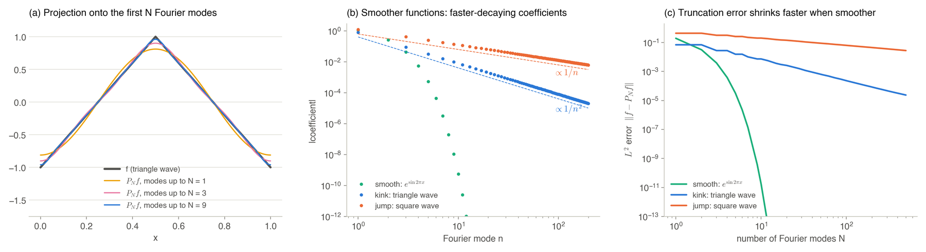
In infinite dimensions a closed, bounded set need not be compact: the basis vectors all lie on the unit sphere, at distance from each other, so no subsequence converges. Smoothness restores compactness, since a ball of smoother functions, , is compact in the norm when , which is the Rellich–Kondrachov theorem: by the inequality above, every function in it lies within of the finite-dimensional space . The quantitative version of compactness is the covering number , the number of balls of radius needed to cover the set, and our error decomposition uses it.
Some natural spaces of functions have a norm but no inner product, such as the continuous functions with the maximum norm, or the paths of finite -variation that we will meet with signatures. A complete normed space is a Banach space, and the tools that rely on inner products, such as orthonormal bases, projections and the Gaussian measures of the next section, do not carry over to it directly, which is why it matters that our first theorem holds on Banach spaces.
Random functions and Gaussian measures
A generative model for functions is a probability distribution on a function space, and probability in infinite dimensions has one big surprise that shapes everything that follows: there is no uniform measure, and so there are no densities. In a probability density is defined relative to volume, the Lebesgue measure, which is the same everywhere, but on an infinite-dimensional space no such measure exists. The reason fits in one sentence: the unit ball contains infinitely many disjoint balls of radius , centered at for each basis vector , and a translation-invariant measure would have to give them all the same mass, so either everything has mass zero or the unit ball has infinite mass. A “density” then only makes sense relative to another measure: has a density with respect to , its Radon–Nikodym derivative, exactly when is absolutely continuous with respect to , written , meaning that every set of -probability zero also has -probability zero.
The best-understood distributions on a Hilbert space are Gaussian. A Gaussian measure is a distribution under which every linear measurement is a one-dimensional Gaussian, with mean and variance . The covariance is a positive, symmetric operator with eigenpairs , and it must be trace class, , for a reason given by the Karhunen–Loève expansion, the infinite-dimensional version of “a Gaussian is a linear map applied to independent standard normals,”
The sum of the eigenvalues is the expected squared size of a sample, so it must be finite for samples to be functions at all. A Gaussian process (GP) with covariance kernel is the Gaussian measure whose covariance operator is , and a smooth kernel gives fast-decaying eigenvalues and smooth samples.
White noise is the case , with for every . The sum diverges, so white noise is not a random element of : on a fixed grid it looks harmless, but its variance is spread evenly over all modes, so it gets rougher as the grid is refined and never settles down to a function. FFM uses GP noise, while kFFM treats the noise distribution, called the base measure, as part of the configuration chosen for each dataset, a GP where the data are smooth and white noise on the grid where the data are rougher than a smooth GP prior, as in the Navier–Stokes family.
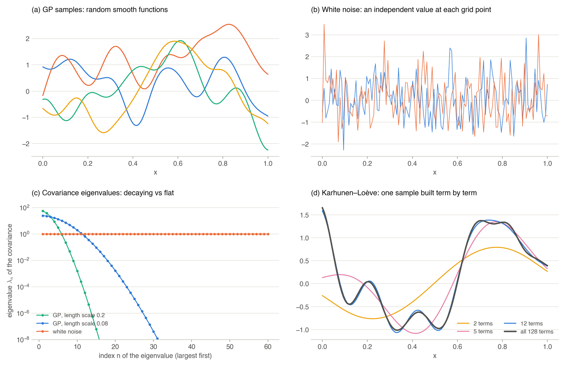
In finite dimensions any two non-degenerate Gaussians have densities with respect to each other, but in infinite dimensions this fails dramatically, for by the Feldman–Hájek theorem two Gaussian measures on a Hilbert space are either equivalent, each absolutely continuous with respect to the other, or mutually singular, living on disjoint sets, with nothing in between. The reason shows up already in high dimensions: under the normalized squared length concentrates at 1, under at 1.21, and as grows the overlap vanishes, so that in infinite dimensions scaling the covariance by any constant other than 1 produces a singular measure.
The Cameron–Martin theorem treats shifts. Moving by a function gives an equivalent measure exactly when belongs to the Cameron–Martin space , the shifts with a finite Cameron–Martin norm , where , and the density is then , where is a linear functional determined by . For a Brownian bridge, the Cameron–Martin space consists of the functions that vanish at both ends and have a square-integrable derivative, so that a smooth shift is allowed and a rough one is not. Samples of the measure itself almost surely lie outside its Cameron–Martin space, since Brownian paths have no derivative at all, so a sample of the noise is never an allowed shift.
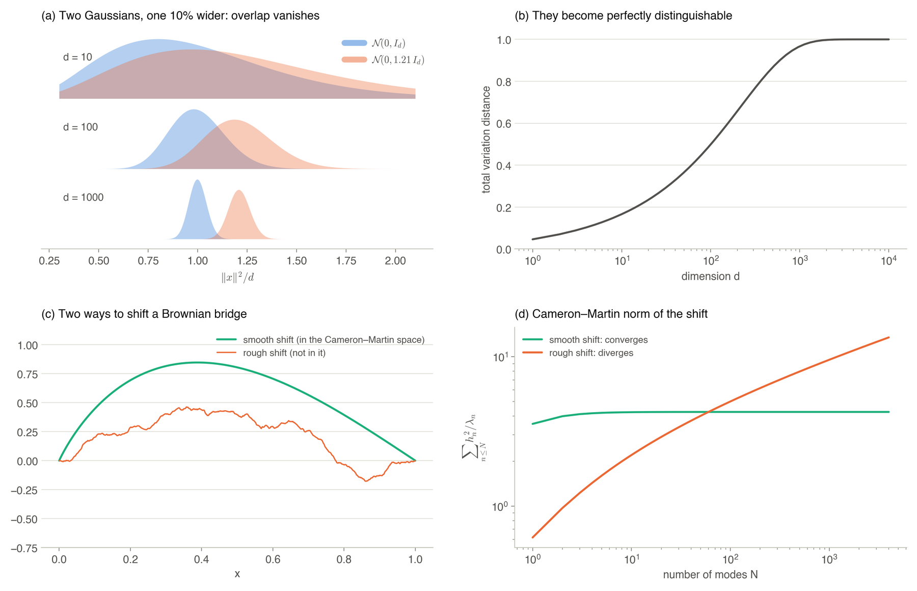
Three consequences recur in the rest of the post. Many tools of optimal transport in use densities with respect to volume, which are not available on function spaces, so we will need a formulation that works with samples and costs alone. FFM’s training loss is justified by an absolute-continuity condition, which requires that at each time each conditional path distribution be absolutely continuous with respect to the mixture of all of them; a sufficient condition is that the data lie in the Cameron–Martin space of the prior, with , and when the data are rougher than the prior this degrades, which is one reason to match the roughness of the base measure to the data, and why white noise is selected on the Navier–Stokes family. And kFFM changes the pairing but inherits this structure, which, as we will see, requires the entropic regularization of optimal transport.
Flow matching, from vectors to functions
We write for the noise or base distribution, or for the data distribution, for a noise sample and for a data sample, and a coupling of and is a joint distribution of pairs whose two sides are and . In , flow matching learns a velocity field , a neural network that says, at every location and time , in which direction and how fast a point should move, and to generate a sample one draws noise and follows the velocity field from to ,
Training is simple: take a noise sample and a data sample , connect them by a straight line, , and teach the network that at the point the velocity should be ,
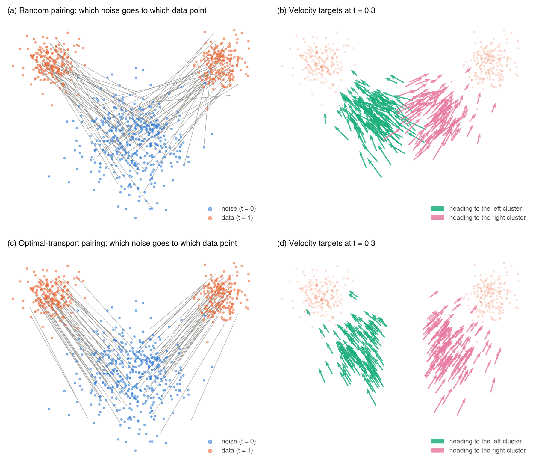
Which noise sample goes with which data sample? The standard answer is any, at random, which is the independent coupling , but flow-matching theory says that the learned flow carries the noise distribution to the data distribution for any coupling, so we are free to choose a better one. Random pairing has a cost: straight lines heading to very different data points pass through the same location at the same time, the network can output only one velocity there, and since the minimizer of a squared loss is the average of the targets, it learns a compromise that points toward none of them. Optimal-transport pairing, introduced for flow matching by Tong and colleagues and by Pooladian and colleagues, pairs each noise point with a nearby data point instead, so that the lines stop crossing and the targets at each location agree.
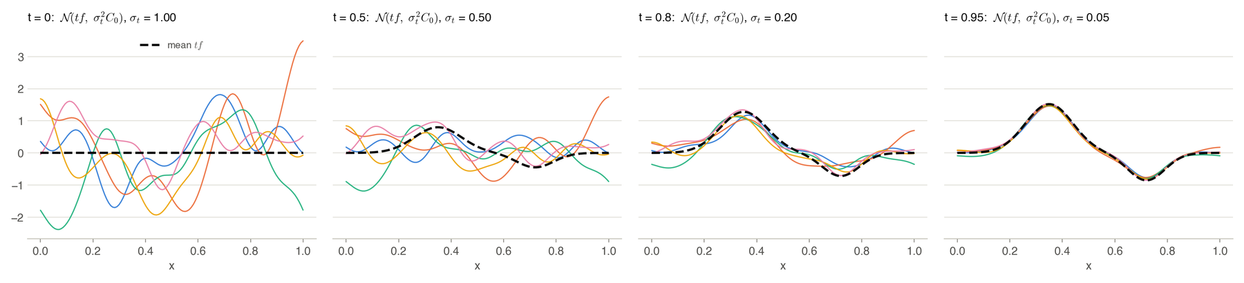
Functional Flow Matching, by Kerrigan and colleagues, carries this recipe over to functions using Gaussian measures. The noise is a Gaussian measure , and for each data function a Gaussian bridge moves the noise toward ,
so that is the prior and is concentrated around . Averaging the bridges over the data, , gives a path of distributions from the prior to, essentially, the data. A sample of the bridge is with , and its velocity is
The network is trained to match this conditional velocity with the loss , and the absolute-continuity condition above is what makes this equivalent to matching the intractable velocity of the averaged path. Within each bridge, the path is already the optimal transport between the two Gaussians and ; what remains random is which data function each noise sample is bridged to, since the endpoint pairing is independent.
The velocity field takes a function and returns a function, so the network is a neural operator. FFM uses a Fourier Neural Operator (FNO), whose layers act on the Fourier coefficients of their input, each computing , where is the Fourier transform and holds learned weights for the lowest modes only. Because the parameters are attached to Fourier modes rather than to grid points, the same network can be evaluated on a finer grid than the one it was trained on.
The problem: random pairs make a hard regression
Writing the bridge with an explicit noise partner shows where the difficulty lies. kFFM uses the same path as FFM, , with the pair drawn from a coupling and the target velocity , which for the independent coupling is exactly FFM. Up to the tiny term, the network regresses the residual between a data function and its noise partner, and under random pairing this residual is the difference of two unrelated draws, a large target that varies a lot from pair to pair, so that the network has to discover the shared structure of the dataset and match each particular instance at the same time. The fix suggested by the two-dimensional picture is to pair each data function with a noise function that is already close to it in a meaningful sense, so that the bridge mostly transports the remaining difference, and the cover figure at the top of this post shows the effect on a synthetic dataset, where the kFFM coupling makes the residuals about 21% smaller on average.
In finite dimensions OT pairing is well established, but in function space it meets two obstacles. The first, as we have seen, is that OT tools relying on densities are unavailable. The second is the choice of distance. The obvious shortcut is to flatten each discretized function into a long vector and use the ordinary squared distance, which is what a direct port of finite-dimensional OT flow matching does and is one of our baselines, CFM-OT(), but a flat distance treats grid values as unrelated coordinates and does not see smoothness, derivatives or path roughness, which are exactly what distinguish one function-valued sample from another. The next four sections develop the tools that address both obstacles: optimal transport computed from samples, kernels that encode the geometry, the divergence that combines them, and the signature kernel for paths.
Optimal transport
Given two distributions and and a cost of moving to , Monge asked in 1781 for the map that pushes onto , written and meaning that if then , at the least average cost . On the real line with a convex cost the answer is to match quantiles, , where denotes a cumulative distribution function, and the optimal map never crosses itself.
A map cannot split mass, however: if puts mass on a single point and spreads mass over three, no map works. Kantorovich replaced maps by couplings, joint distributions on pairs whose two sides are and , and posed
With for a metric , is the Wasserstein distance, a metric on distributions, and the quadratic case is the reference our error decomposition compares against. An optimal coupling exists whenever the spaces are Polish, that is, complete and separable metric spaces, and the cost is lower semicontinuous and bounded below; separable Hilbert spaces and the path spaces we use are both Polish, so the problem is well defined on them. The problem also has a dual form, , whose optimal functions are called potentials.
Adding a penalty that keeps the plan spread out,
makes the problem strictly convex and gives the optimal plan an explicit form, a density with respect to the independent coupling,
for two potentials . The Sinkhorn algorithm finds them by alternately fixing each marginal, setting and then the same for . On a minibatch of noise and data functions everything becomes a matrix, the cost matrix , the Gibbs kernel , and a plan whose rows and columns each sum to , and Sinkhorn alternately rescales the rows and columns of . The regularization sets how soft the plan is, and training pairs are then sampled from the plan.
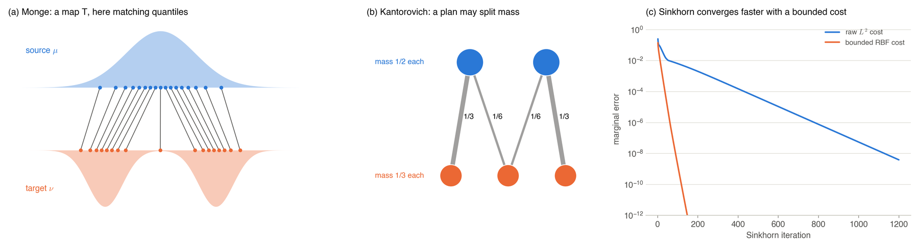
The right-hand panel previews a point that becomes our first theorem. When a few pairs have enormous costs, the entries of span many orders of magnitude and Sinkhorn converges slowly, whereas a bounded cost keeps bounded away from 0 and 1, and convergence is fast regardless of outliers.
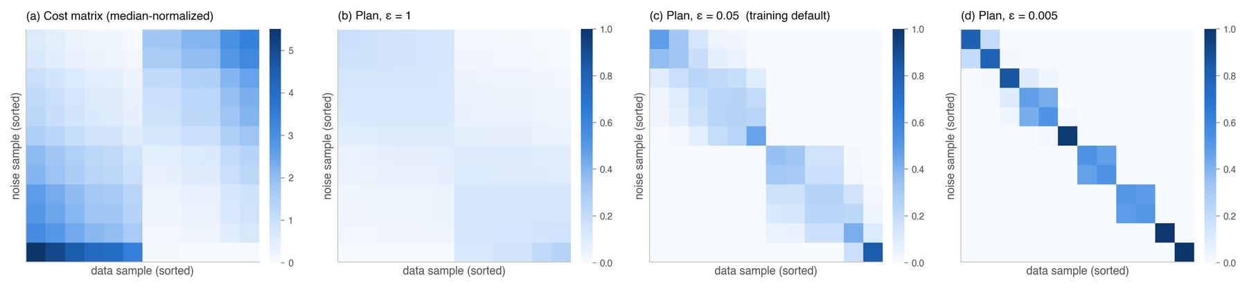
Two facts make minibatch entropic OT practical in function space. It needs only the cost matrix, since Sinkhorn never asks for a density, only for the pairwise costs, which sidesteps the first obstacle and leaves the choice of cost. And minibatch plans are a valid coupling: averaged over batches, they define a coupling of the true noise and data distributions, as Fatras and colleagues showed in their analysis of these “expected minibatch plans,” so the flow-matching guarantee still applies, the batch size changes only which pairs are used, and as it grows the plan approaches the full entropic OT plan. In practice a few choices matter for stability, and we recommend them as defaults: dividing each batch’s cost matrix by its median, the most important one since it makes scale-free, running Sinkhorn in the log domain, using , and sampling pairs from the plan rather than averaging over partners.
Because of the entropy term, , so a distribution is not at zero distance from itself. The Sinkhorn divergence removes this bias,
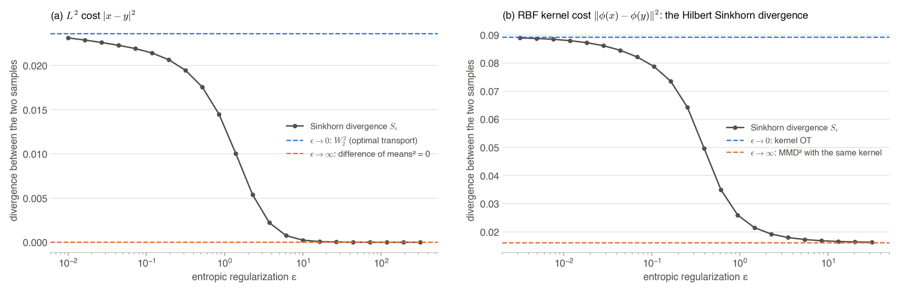
and, as Feydy and colleagues showed, it interpolates between optimal transport as and a kernel discrepancy, an MMD, as . We will see what this interpolation looks like with a kernel cost once kernels are in place.
Kernels, RKHS and MMD
A positive-definite kernel is a symmetric similarity score whose matrices are positive semidefinite for every finite set of points, and every such kernel comes with a Hilbert space of functions, its reproducing kernel Hilbert space (RKHS) , in which evaluating a function at a point is a continuous operation. By the Riesz representation theorem, evaluation at is an inner product with a special element ,
The map is the feature map, which turns each point into a function, and inner products of features are kernel evaluations, so the features never need to be written down, which is the “kernel trick.”
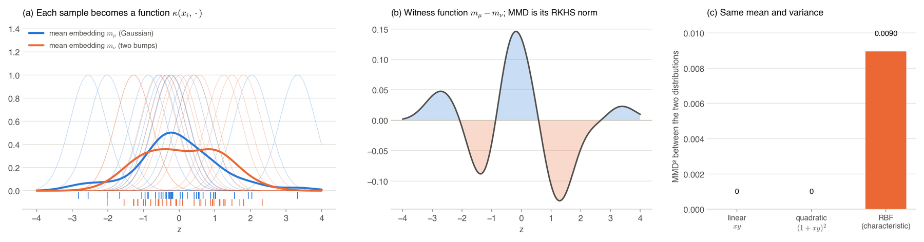
Averaging the features gives the kernel mean embedding of a distribution, , a single element of the RKHS, which exists for every distribution exactly when the kernel is bounded, one more reason boundedness will matter. The distance between embeddings is the maximum mean discrepancy (MMD),
with and independent. Equivalently, , the largest difference in expectation over smooth test functions, whose best test function, the witness, is proportional to . MMD needs only samples, which is why it is our main evaluation metric, and its unbiased estimator drops the terms where a sample is compared with itself, so it can be slightly negative when two distributions are close, as some values in our results are.
MMD is a true distance between distributions only if the embedding is injective, that is, if implies , and such kernels are called characteristic. A linear kernel only compares means, and a quadratic one means and variances, while the Gaussian or RBF kernel is characteristic on every separable Hilbert space, as Ziegel and colleagues showed, so the RBF kernels we use on and on Sobolev spaces are characteristic. Universal kernels, whose RKHS can approximate every continuous function on a compact set, are characteristic too, and the signature kernel is universal on compact sets of time-augmented paths.
Every kernel defines a squared distance between points, the squared distance between their features,
and the plain inner product gives back the cost. kFFM uses three kernels on function spaces. The Euclidean RBF, , gives , which for nearby pairs is approximately and so keeps the ranking, while for distant pairs it levels off at 2, so that outliers cannot dominate; its bandwidth is set by the median heuristic. The Sobolev RBF is the same kernel with the norm replaced by the Sobolev norm , which also compares derivatives, so that fast wiggles count. And the third is the signature kernel for paths, to which we come shortly.
The Hilbert Sinkhorn Divergence
Li and colleagues combined the two preceding ideas, embedding both distributions in the RKHS with the feature map, and , and comparing the embedded distributions with entropic optimal transport under the squared RKHS distance,
The Hilbert Sinkhorn Divergence (HSD) is its debiased version, , computed in the RKHS. The features may be infinite-dimensional, but by the kernel trick the whole problem can be solved on the original space with the kernel-induced cost , since the optimal plans correspond to each other under the feature map and the divergences are equal, so that the HSD is entropic OT under the cost , and its plan is exactly the coupling kFFM uses.
The interpolation between OT and MMD takes a clean form here. As , the HSD tends to optimal transport between the embedded distributions, kernel OT; as , the plan tends to the independent coupling, and the debiased divergence becomes
because the terms cancel. Both ends are genuine distances between distributions when the kernel is characteristic, whereas with the plain squared cost the large- end is only the squared difference of the means, which is blind to everything else.
In our paper the HSD is the object of analysis, what the theorems control, while training uses only its plan, since the two debiasing terms do not depend on the coupling and cannot change which plan is optimal. Li and colleagues established its statistical consistency and finite-sample bounds for vector data, and our theorems extend the setting to function spaces.
Paths and the signature kernel
Time series are paths, and paths have structure that neither nor Sobolev norms capture well, namely the order in which things happen and how rough the path is. A path is a continuous map , and its roughness is measured by its -variation, , the supremum over all partitions of . Paths of finite -variation form a Banach space; we work with , for which the integrals below are classical Young integrals, and treat a discrete time series as the piecewise-linear path through its observations.
The signature of a path is the sequence of its iterated integrals,
where lies in . The first level is the increment, , and the second is a matrix whose symmetric part is fixed by the increment, , and whose antisymmetric part is the Lévy area, , the signed area between the path and the straight chord from its start to its end, while higher levels record higher-order interactions between the coordinates. Three properties make the signature a good feature map for paths. It ignores speed and position and sees shape and order, for it does not change if the path is traversed faster or slower or is translated; without extra information it identifies a path only up to “tree-like” detours that retrace themselves, but adding time as a coordinate, , removes this ambiguity and makes the signature sensitive to timing, and we always use this time augmentation. It decays factorially, , where is the length of the path, so truncating at a moderate level loses little. And it is universal, since on compact sets of time-augmented paths linear functions of the signature approximate every continuous function of the path, just as polynomials approximate continuous functions on an interval. The signature of a concatenation of two paths is the tensor product of their signatures, a fact called Chen’s identity, and it is how the signatures in the figures below were computed, one linear segment at a time.
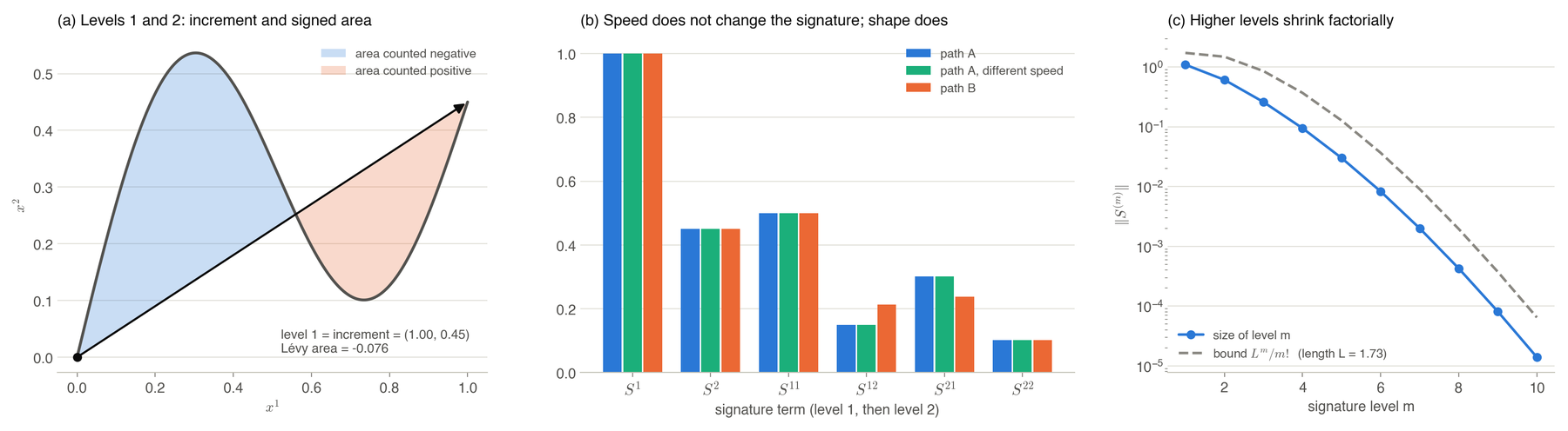
The signature kernel is the inner product of two signatures over all levels,
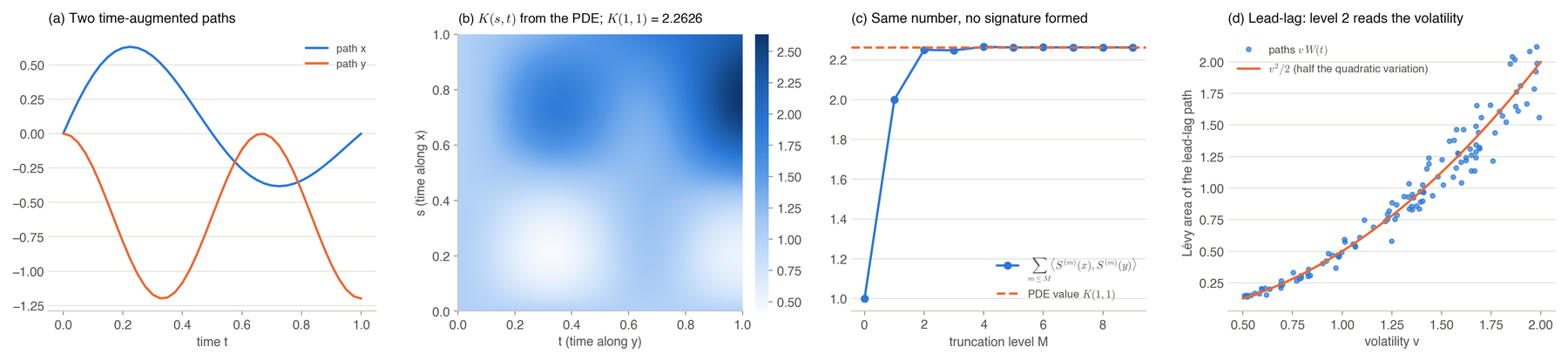
and computing it does not require forming the signatures, whose size grows like . Salvi and colleagues showed that , the kernel between the two paths stopped at times and , solves
which for smooth paths is the hyperbolic Goursat PDE with on the two axes. The kernel is , obtained with a standard finite-difference solver, and we use the pySigLib library. Two hyperparameters of this computation appear in our sensitivity study, the refinement of the PDE grid, called the dyadic order, and the bandwidth of a static kernel through which the increments can first be passed, and since the solver’s grid has one cell per pair of time steps, memory grows with the product of the two path lengths.
For a one-dimensional series, the lead-lag transform pairs the path with a copy of itself delayed by one step, and the Lévy area of the resulting 2D path equals half the sum of squared increments, the path’s quadratic variation, which measures its volatility. This is how the signature kernel tells a calm path from a jittery one even when their overall trends match, something the distance cannot do, as the toy examples below show.
kFFM on one page
kFFM is FFM with one step changed. Each training iteration draws a batch of noise functions , from a GP or white noise, and data functions , and computes the kernel cost matrix
which it divides by its median. It then runs log-domain Sinkhorn with to get the plan , samples pairs from , draws a time uniformly in and forms , and finally regresses the network output onto the target with a squared loss and takes a gradient step.
The kernel enters at exactly one place, the cost matrix. No sample is mapped into the RKHS: the neural operator sees the original discretized functions, the paths are built in the original space, and generation is unchanged, starting from noise and following the learned velocity, so that if the plan is replaced by random pairing the algorithm is exactly FFM. The kernel should match the data class, the signature kernel for path-like data, the Sobolev or Euclidean RBF for smooth fields, where the Euclidean RBF is a reasonable default, and RBF or costs for very long paths, where the memory of the signature kernel becomes the bottleneck.
Two toy examples where flat pairing fails
Before the benchmarks, we ran a controlled test of the two weaknesses of the cost, that it is unbounded and that it is blind to structure. We draw sources and targets that have an intended matching, sort both so that the intended matches lie on the diagonal, compute the entropic plan under each cost exactly as in training, with and median-normalized costs, and report how much of the plan’s mass falls on the intended matches, where a uniform plan scores about 0.14 to 0.19.
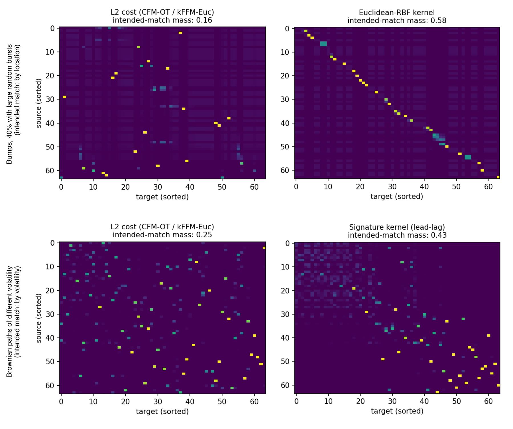
The top row shows a conditioning failure. The burst pairs dominate the median normalization of the unbounded cost, the contrasts between clean pairs fall below , and the plan is close to uniform, with 0.16 of its mass on the intended matches, while the bounded RBF cost saturates the bursts and recovers the matching (0.58) whatever the burst amplitude, and any bounded cost would fix this. The bottom row shows a geometry failure. For two independent Brownian paths with volatilities and , the expected cost is , which does not depend on whether and are similar, so it carries no signal about the intended matching and the plan stays close to uniform (0.25), whereas the signature kernel reads volatility through the quadratic variation and concentrates on the intended matching (0.43), and only the change of geometry fixes this. The full figure in the paper also shows that no single cost wins every scenario, since the signature kernel, for example, fails on the burst example, which is why kFFM chooses the kernel per data class.
What the theory says, and what it does not
With the background in place, the three theorems can be stated almost as in the paper. They certify the kernel pairing; they do not, by themselves, explain why sample quality improves, which is an empirical claim tested in the results.
Theorem 1, on well-posedness and uniform boundedness, states that if is a real Banach space and a bounded positive-definite kernel on it, with for all , then for all , and for every the Hilbert Sinkhorn Divergence is finite for all pairs of distributions, with . Finiteness alone is not the point, since under a second-moment assumption the cost is integrable too, and for a Gaussian prior . What the theorem adds is a bound that is uniform, with no assumption on the distributions, and that holds without an inner product. The first part conditions the solver, for the Gibbs kernel stays bounded away from 0 and 1 in every batch, so Sinkhorn converges regardless of outlier pairs, and we measured the bounded RBF cost to be about 8 times faster per batch than the unbounded cost at . The second part covers path spaces, which are Banach but not Hilbert, and therefore licenses the signature kernel, our strongest configuration.
Theorem 2 is an error decomposition. Let be a compact metric space of diameter , let be optimal transport with the quadratic cost , and let be the largest gap between the kernel cost and the squared distance; then for every and ,
where is the covering number. The compact spaces are the ones built earlier, Sobolev balls inside for , and compact sets of paths for the signature kernel. The entropic and covering terms vanish as and go to zero, but the mismatch term is irreducible, since more samples or finer grids do not shrink it. For the RBF kernel it is small at large bandwidth, because is a rescaled cost up to relative error for batch diameter , and on smooth Navier–Stokes fields the plans under the RBF and costs nearly coincide, at a total variation of at most 0.02. For the signature kernel the mismatch is large by design, since we want a different notion of closeness, and the theorem then controls the deviation from transport with the chosen geometry rather than proximity to transport; the pair rankings differ substantially from , with a rank correlation of 0.33–0.37 on the AEMET and gene-expression data, which is where the largest gains occur. In rough regimes the bound degrades on two fronts, as a smooth kernel cost saturates, enlarging , and the covering number explodes as the effective smoothness approaches the compactness threshold.
Theorem 3 concerns discretization invariance. On a bounded periodic domain , take distributions on the Sobolev ball with , viewed inside , and let be their projections onto the span of about Fourier modes; then for the Sobolev-RBF kernel on and every ,
or in terms of the grid spacing . This is the truncation inequality from the section on function spaces carried through the kernel and the transport problem: the smoother the data relative to the kernel’s norm, the faster the objective computed on a grid approaches the continuum one, which is the formal counterpart of resolution invariance. Combining Theorems 2 and 3 bounds the gap between the objective the model actually computes and continuum quadratic optimal transport in by four interpretable terms, kernel mismatch, entropic blur, covering and discretization, of which only the last vanishes as the resolution grows.
One more property matters: kFFM inherits FFM’s foundations. FFM’s loss rests on absolute-continuity relations between Gaussian measures, and with a bounded cost the entropic plan has a density with respect to the independent coupling, , with bounded potentials, so this density is bounded above and away from zero. The plan is therefore equivalent to the independent coupling, its conditionals are equivalent to the prior, and every absolute-continuity relation that FFM relies on transfers to kFFM. This is where entropic regularization matters beyond computation, since an unregularized OT plan can be singular with respect to the independent coupling, and the argument would fail.
Finite-dimensional OT flow matching is often motivated by straighter paths and hence cheaper sampling, but we make no straightness or sampling-efficiency claim. kFFM changes only which endpoints are paired, the path between them is the same straight-line template, and the geometry of Gaussian measures on Hilbert spaces, Bures–Wasserstein rather than flat, does not inherit the Euclidean picture behind that intuition, as the paper’s appendix states precisely.
Results
We used four sequence datasets, AEMET (the mean annual temperature profile at 73 Spanish weather stations, 365 points), gene expression, economic series (population, GDP and labor) and volatility paths from the Heston model, and four PDE datasets, the 1D Korteweg–de Vries (KdV) equation, the 2D incompressible Navier–Stokes equation and stochastic versions of both, with a turbulent Navier–Stokes benchmark added at the end. The baselines are FFM; functional diffusion (DDPM); a score-based denoising diffusion operator (DDO with NCSN noise scales); an adversarial neural operator (GANO); and CFM-OT(), which uses the same Sinkhorn solver and neural operator as kFFM but applies OT to the flattened grid with the raw cost and white noise.
The main metric is the MMD with an RBF kernel, computed with the unbiased estimator, so that a tiny or negative value means “indistinguishable from the data at this sample size,” and percentage gains there are not meaningful. Because an RBF-based metric could favor an RBF-based pairing, we also report non-kernel metrics (the sliced Wasserstein distance and the marginal ), structural diagnostics (the autocorrelation error for sequences and the log-spectrum error for PDEs) and physics diagnostics on Navier–Stokes. Results are over 10 seeds (20 for the comparison with FFM on four datasets), and all methods share seeds, so comparisons are paired by seed.
For each dataset, the cost and the base measure of kFFM are chosen on a held-out validation split by sliced Wasserstein distance, a criterion that does not involve the kernels being compared. The selected configurations follow the rule given above: the signature kernel with a GP base on path-like data, except short-horizon Heston, where the top configurations are statistically indistinguishable and the rule picks the RBF cost with white noise; the Sobolev-RBF cost with a GP base on the KdV family; and the Euclidean RBF cost with white noise on the Navier–Stokes family, whose rough fields a smooth GP prior matches poorly.
Distributional quality
kFFM has the lowest MMD of all six methods on all eight datasets. Where the strongest baseline is not at the noise floor, the improvement over it is 74% on stochastic KdV, 60% on Economy and on gene expression, 34% on stochastic Navier–Stokes and 8% on Navier–Stokes, and relative to CFM-OT(), the same solver and network with a flat cost, kFFM lowers MMD by 75% on gene expression and 66% on Economy.
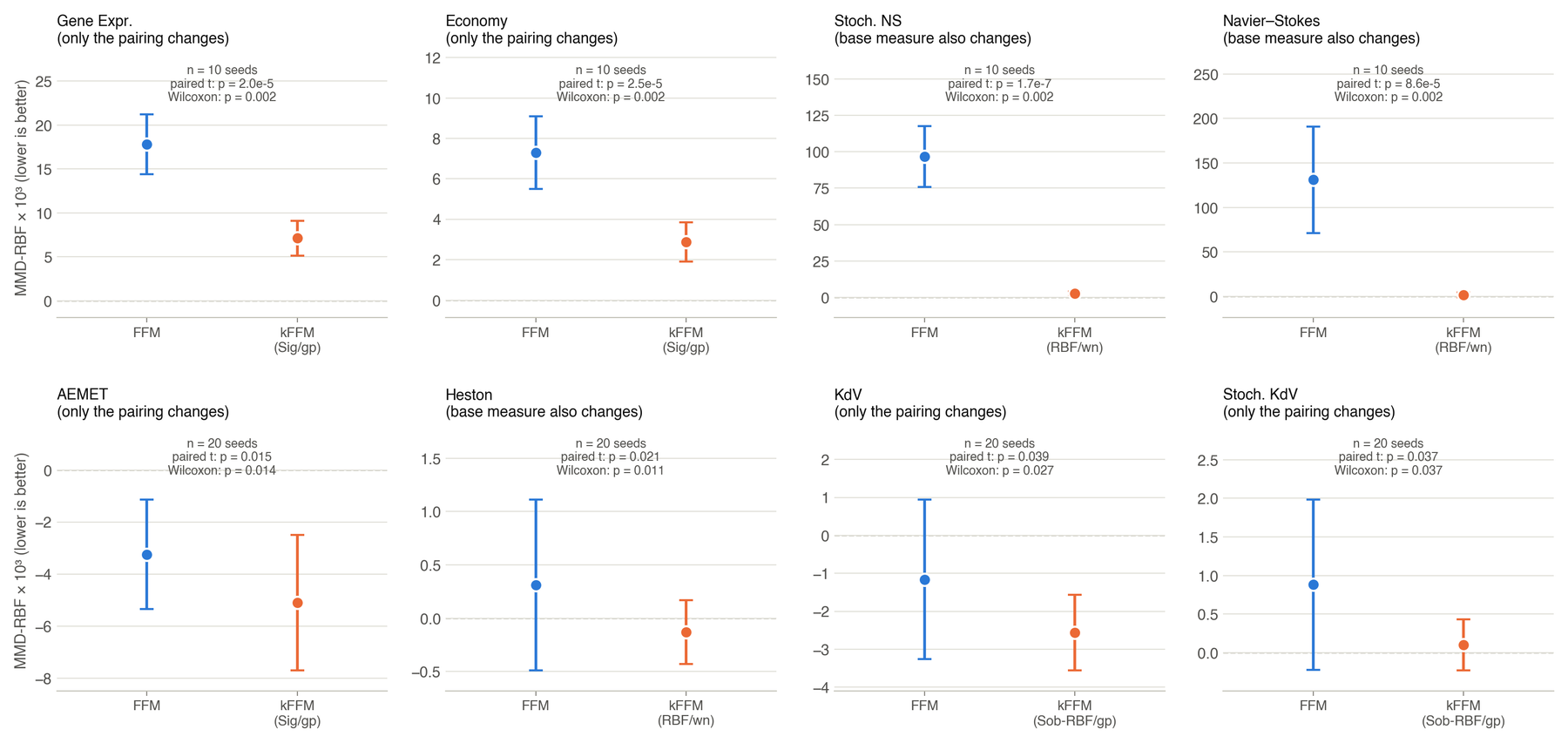
kFFM improves on FFM on every dataset at the 0.05 level under both tests, and on the four datasets with the largest gaps it wins on every seed. The evidence is not equally strong everywhere, however: on AEMET, Heston, KdV and stochastic KdV the MMD values sit near zero and the p-values are between 0.011 and 0.039, significant but modest.
On the same runs, kFFM also improves the sliced Wasserstein distance and the marginal over FFM on the four datasets of the paper’s non-kernel table, by 18–20% on gene expression and Economy, where each comparison is significant when paired by seed, and by 2.9–4.1× on Navier–Stokes and stochastic Navier–Stokes; for the signature configurations the pairing kernel and the evaluation kernel already differ. The structural diagnostics show what MMD understates, for CFM-OT() matches pointwise values reasonably well but has 105× and 66× larger autocorrelation error than kFFM with the signature kernel on Economy and gene expression, and function-level structure is where the kernel pairing helps most.
Bounded cost or function-space geometry?
Both effects isolated in the toy examples show up on real data, on different data classes.
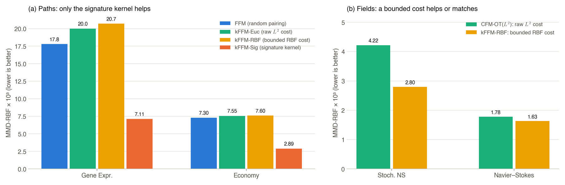
On paths, geometry is what matters, for no Euclidean cost recovers the gains of the signature kernel: on gene expression, kFFM with the raw cost reaches 20.0 and with the RBF cost 20.7, against 7.11 with the signature kernel, and on Economy 7.55 and 7.60 against 2.89, so the signature kernel genuinely re-ranks pairs relative to . On smooth fields, boundedness is what matters, since the RBF cost is a monotone transform of , with the same ranking of pairs and the outliers compressed, and on smooth Navier–Stokes fields the plans under the two costs nearly coincide, at a total variation of at most 0.02. What the bounded cost buys there is conditioning, robustness to and faster Sinkhorn, and it matches or improves the unbounded cost at the same base measure.
A turbulent stress test
The Navier–Stokes benchmark above is smooth, the regime where our theory is informative. To test the rough regime, where Theorem 2 is weakest, we used the turbulent 2D Navier–Stokes benchmark of the FNO paper (viscosity , Reynolds number about 2000) and compared seven methods over five seeds, with the same network and training budget for all. Besides MMD and the sliced Wasserstein distance, we measured physics diagnostics: the distributions of vorticity and enstrophy, the skewness and kurtosis of the vorticity, and the energy spectrum.
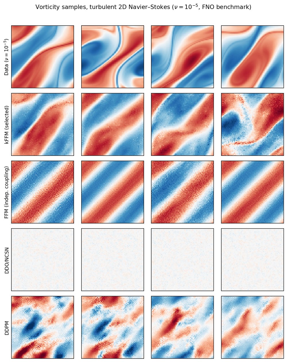
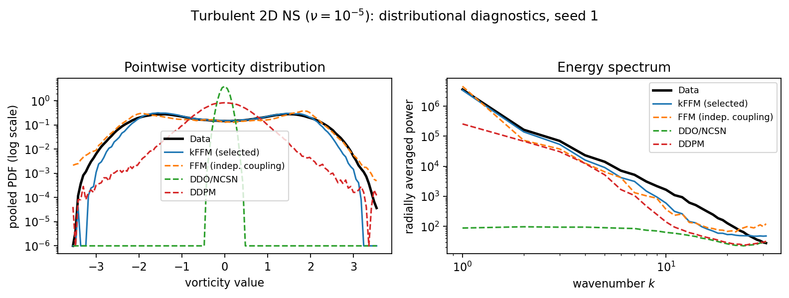
kFFM has the best value on five of the seven metrics and ties for the best MMD, while CFM-OT() at the same white-noise base overlaps with kFFM within one standard deviation. OT-paired flow matching is far more robust than the score-based and diffusion alternatives, with 23–32× better vorticity-distribution , 5.7–6.9× better enstrophy , and 17–43× smaller kurtosis error. Against FFM with its GP prior, kFFM improves every metric except kurtosis, where the two tie, with seed-paired significance (its MMD, for example, is 73× lower, ). This gain combines two changes, however: the three methods that use the GP base are indistinguishable from each other, so in this regime the white-noise base does most of the work, and at that base the kernel and raw costs tie. The turbulent benchmark therefore supports OT-paired flow matching with a white-noise base as the strongest current option, without singling out the kernel cost.
Cost and sensitivity
The per-batch Sinkhorn solve adds 5–7% to end-to-end training time at the largest resolution we train, Navier–Stokes. Its cost grows with the square of the batch size but does not depend on the model size or the resolution, so its share shrinks as the network grows; peak memory for the pairing is 80–151 MB, 1.5–9% of the network’s own peak, and one pairing takes about as long as one network step. The bounded RBF cost makes Sinkhorn about 8 times faster than the raw cost at (9 against 73 ms per batch) and training 15–25% faster end-to-end, and giving FFM the extra time as additional epochs does not close the gap.
Results are indistinguishable within seed-to-seed variation for RBF bandwidths between 0.1 and 2. With bounded costs they barely move across the Sinkhorn regularization values we swept, whereas the raw cost degrades by about 10× at on long volatility paths, and they are unchanged across the signature kernel’s dyadic order (0 to 3) and static bandwidth (0.1 to 5). The kernel family is the choice that matters: match the kernel to the data class, set the bandwidth by the median heuristic, and validate with a non-kernel metric on held-out data. The properties the theorems require, boundedness and characteristicness, hold for every kernel we consider, so the theory constrains the family only weakly and the selection rule does the rest.
Limitations
The theory certifies the pairing, not the samples: it establishes well-posedness, an error decomposition and discretization invariance, but says nothing about straightness or sampling speed, on which we make no claim, and the gains in sample quality remain an empirical finding. Rough data are where the theory says least, for on the turbulent benchmark the distances between noise and data functions more than double relative to the standard benchmark (a median of 91 against 40), which pushes the RBF cost into saturation, so that the mismatch term grows and the covering term of Theorem 2 is large for any practical , and there the empirical results carry the method. Turbulence is still open, since the failures sit mainly with the score-based and diffusion baselines, but all methods, ours included, leave headroom (the best sliced Wasserstein distance is 0.19), and in this regime the base measure rather than the pairing does most of the work. The signature kernel is memory-hungry on long paths, its memory growing with path length (0.63 GB at 100 time points against 12.5 GB at 512), so very long paths fall back to RBF or costs. And some gains are modest, for on four datasets the MMD values are near the noise floor and the paired p-values are between 0.011 and 0.039.
Takeaways
Pairing is a design choice: flow matching works with any coupling of noise and data, random pairing is the default rather than a requirement, and pairing each data function with a noise function that already resembles it leaves the network a smaller, more structured residual to learn. In function space, transport needs samples rather than densities, for without a uniform reference measure densities and many classical OT tools are unavailable, but minibatch entropic OT needs only pairwise costs, and its plan keeps the absolute-continuity structure that FFM relies on. A kernel is the way to choose the geometry, bringing prior knowledge about the data into the pairing, since bounded costs keep Sinkhorn well conditioned, Sobolev norms see derivatives, and the signature kernel sees the order and roughness of paths, while the resulting Hilbert Sinkhorn Divergence sits between kernel OT and MMD. And the change is cheap and leaves everything else alone, adding 5–7% to training at our largest resolution without touching the network, the loss or the sampler. If you generate time series, paths or PDE fields with flow matching, we hope kFFM is a useful drop-in change, and the code is on GitHub.
This work was partially supported by NSF 2303037, NSF 2312501, NSF 2531008, NSF 2553619, SRC JUMP 2.0 Center, CDSC Industry Partners, Amazon Research Awards, Snapchat, and Google Gifts. Barbora Barancikova is supported by UK Research and Innovation [UKRI Centre for Doctoral Training in AI for Healthcare grant number EP/S023283/1]. Part of this work was done while Fred Xu was an intern at Block, Inc., and we thank Block, Inc. for its support. The toy-coupling panels are cropped from a figure in the paper, and the turbulent samples and statistics are from the paper; the other figures were made for this post, with synthetic examples except for the paired-test and cost charts, which use the numbers in the paper.